A Comparison of Heritability Estimators in Brain Imaging

Shen Ting Ang^[1], Xu Chen^[2] and Dr Thomas Nichols^[3], Department of Statistics, University of Warwick

Abstract

Studies of twins can be used to estimate heritability - the proportion of variability of a phenotype which can be explained by genetic causes. Methods of quantifying heritability include Falconer's estimate, Restricted Maximum Likelihood (ReML) and Bayesian methods. Functional Magnetic Resonance Imaging (fMRI) is an established tool used to understand how the brain works, but the heritability of fMRI measures is not well established. The purpose of this work is to investigate the three heritability methods with respect to potential use with fMRI data. We considered the performance of the methods at a single voxel (volume element) alone, and in the case regularising over a set of adjacent voxels. We found substantial differences in the performance of these methods, with Falconer's exhibiting much greater bias and variance properties. Simulation results show lower computing times, lower variance and increased bias with Bayesian methods. It is hoped that these results can be used for comparison with further studies, with the ultimate goal of developing methods for real fMRI data.

Keywords: fMRI, Twin studies, Heritability, Bayesian, Restricted Maximum Likelihood, neuroimaging statistics, SPM

Introduction

Heritability is an essential tool used to measure the genetic influence over quantitative traits. No collection of DNA is required, but related individuals must be measured and typically only monozygotic (MZ, "identical") and dizygotic (DZ, "fraternal") twins are considered. While there are several different measures used for quantifying heritability (Griffiths, 2000: 655-82), the most common is narrow-sense heritability h², the fraction of phenotypic variation that is explained by additive genetic variation. There are different methods of estimating h²(Bellera, 2001: 3-18), and we will consider three of them below.

Functional Magnetic Resonance Imaging (fMRI) has emerged as the popular choice for studying the brain. Data obtained from fMRI studies of twins can be and has been used to study brain development and heritability, such as in the work by Schmitt (2008). Using generated simulated fMRI data, we perform repeated Monte Carlo simulations using the SPM8 package to investigate the effectiveness of different methods of estimation and data smoothing in predicting the model of heritability. The estimators considered are (a) Falconer's Estimate, (b) Restricted Maximum Likelihood (ReML), (c) Bayesian variance components. We describe each in turn below.

It is hoped that the results obtained will provide a better idea of the performance of various methods for further analysis on simulated data in higher dimensions with the ultimate aim of refining methods for analysis on real fMRI data used in heritability twin studies.

Methods

In our study of twins, a fixed linear model and the classical ACE model was deployed, where the fixed linear model is the marginal model of a linear mixed model and can be described as

$Y = X\beta + \varepsilon, {\varepsilon}\sim{N(0, V)}$

The classical ACE model breaks down the observed variance V into variance of genetic (α²), non-genetic familial (c²) and unique environmental (e²) (Neale and Maes, 1994). ReML is a method for estimating variance components that accounts for the degrees of freedom and thus should have less bias than maximum likelihood (Searle, 1992: 159).

SPM8

Statistical Parametric Mapping (SPM) is a free package developed by members and collaborators of the Wellcome Trust Centre for Neuroimaging. It is used for the analysis of brain imaging data sequences, such as for fMRI data. The latest version of SPM is SPM8 and this is the version used for all the simulations below.

SPM uses a voxel-based approach with parametric statistical models. It uses a variant of ReML with Bayesian priors on the variance parameters (Friston et al., 2007: 613-17). Whether classical ReML or Bayesian ReML, the variance components approach uses the same likelihood as used in Structural Equation Models approach to heritability estimation, such as that used by Rijsdik and Sham (2002).

Falconer's Estimate

Falconer (1996: 112-33) proposed the estimator of h²which is perhaps most widely used. The assumptions are equal action of the environment on twins, and dizygotic twins having half their genetic background in common, and thus we get the following as demonstrated by Bellera (2001: 14):

h²= 2(ρ_MZ - ρ_DZ) where ρ_MZand ρ_DZdenote the sample correlation of identical and fraternal twins respectively.

As with other less commonly used estimators, many limitations exist. Bellera (2001: 3-17) gives an overview of various estimators used and gives arguments for and against each of them, but there is no clear conclusion as to which is best. For the purposes of this study, we choose to use Falconer's as a comparison against the other methods.

Restricted Maximum Likelihood (ReML)

Restricted Maximum Likelihood (ReML) was originally introduced in the 1970s and used for mixed models. Later work saw ReML being used for General Linear Mixed Models and Generalised Linear Mixed Models (GLMM) as well. The full details of ReML are not in the scope of this paper; however, both Kneib (2003) and Searle (1992: 158-59) give the full details of this method. ReML can be thought of as the modified maximum likelihood estimation (MLE), which applies MLE on the residuals of the considered model to estimate the parameters. ReML is better than MLE because ReML takes into account the loss in degrees of freedom, which produces the unbiased estimators for the parameters. ReML calculations are usually tedious and require the use of large amounts of memory and processing time to compute (Kneib, 2003). In our simulations, we use two different implementations of ReML - invoking the SPM package and a direct implementation. The main difference is the lack of an Expectation Maximization (EM) step in the direct implementation (Friston et al., 2007: 282-83).

Bayesian Estimation

Bayesian estimation is an approach based on Bayes's Theorem of conditional probabilities:

$P(A|B) = \frac{P(B|A)P(A)}{P(B)}$

The main result of Bayesian estimation is well-known, as given in Searle (1992: 94) amongst many others:

$\pi(\theta|y) = \frac{f(y|\theta)\pi(\theta)}{\int_{R_{\theta}}f(y|\theta)\pi(\theta) d\theta}$

where $\pi(\theta|y)$ is the posterior density for the parameter $\theta$ occurring in the density function $f(y|\theta)$ , $\pi(\theta)$ is the prior density of $\theta$ and $R_{\theta}$ is the range of possible values of $\theta$ .

Breslow (1990) discusses the advantages of using Bayesian methods such as the simplification of data analysis. In practice, it was noted that Bayesian estimation methods computed significantly faster than non-Bayesian methods, sometimes reducing simulation times by more than 30%. In practice, the 1-dimensional simulations took roughly 3 days for each run, hence the savings in simulation times amounted to about a day.

In practice, we control the "amount" of Bayesian estimation by the hC variable in SPM8 - this variable controls the a priori variance (Friston et al., 2007). The baseline, non-Bayesian case has hC = exp(-8) which was chosen at the suggestion of the authors of the SPM8 package. Part of this study is devoted to exploring the effects of varying the parameter hC and how this affects the results obtained in the simulations.

Simulations

The simulations were coded and done in MATLAB, using the SPM8 Package to handle calculations of ReML and Bayesian estimates (Friston, 2007: 275-94, 613-17). The number of voxels (nV) simulated is 20. The numbers of subjects simulated are 20, 40, 60, 80 and 100 respectively, half representing monozygotic twins and the other half representing dizygotic twins. The scenarios of (a) no heritability, (b) only genetic correlation, (c) only common environment and (d) both genetic and common environment were considered. We were mainly interested in the amount of bias and standard deviation from estimating heritability in each case. The steps were as follows:

Generate a random signal with normal errors.
Given different models of heritability, estimate the heritability using Falconer's method, ReML (through SPM), ReML (direct implementation) and Bayesian Estimation (through SPM).
Calculate the bias, variance and mean square errors of each of the estimators.
At the end of the runs, calculate the proportion of time each model is selected correctly using the various estimators.

The following models of heritability were considered:

No heritability, i.e. full unique environmental correlation (e²)
Only genetic correlation (α²)
Only non-genetic familial correlation (c²)
Both genetic and non-genetic familial correlation (α²) and (c²)

With the exception of the first case, we consider a range of values of correlation in each case.

Results

We first review the results from using SPM8's Bayesian method to Falconer's, and then compare ReML to Falconer's.

SPM8

Figures 1 and 2 show the bias and standard deviation of SPM8's method compare to Falconer's method for a total of 100 subjects, and without and with smoothing. It can be seen that the results are comparable between the baseline and smoothed ReML and Falconer's, but the Bayesian Estimation method gives rise to higher bias, lower standard deviation and higher model selection accuracy.

Figure 1: Comparison of Bias for ReML h2 vs Falconer

Figure 1: Comparison of Bias for ReML h²vs. Falconer's h²and Bayesian h²vs. Falconer's h² across different heritability models.

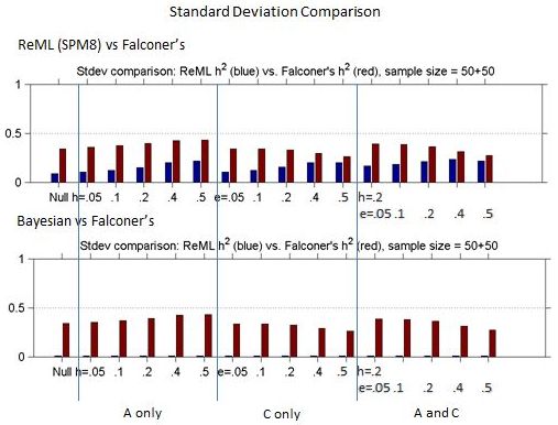
Figure 2: Comparison of Standard deviation for ReML h2 vs Falconer

Figure 2: Comparison of Standard deviation for ReML h²vs. Falconer's h²and Bayesian h²vs. Falconer's h² across different heritability models.

Figure 3: Comparison of Model selection accuracy for ReML vs Bayesian across different heritability models

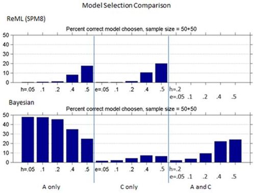
Figure 3: Comparison of Model selection accuracy for ReML vs. Bayesian across different heritability models.

Using ReML without SPM8

Next, ReML without using SPM8 is considered with n_MZ= n_DZ= 50.ReML will be compared with Falconer's and SPM's ReML below, where three kinds of smoothing methods will be applied and compared.

ReML vs. Falconer's

ReML tends to give lower bias and standard deviation as compared to Falconer's. The significant difference between ReML estimate and Falconer's estimate tends to suggest that ReML can be a better method.

(A, C, E)	ReML Bias	Fal Bias	ReML Stdev	Fal Stdev
(0, 0, 1)	0.1767	0.2302	0.0058	0.3372
(0.2, 0, 0.8)	-0.0164	0.1415	0.0065	0.3958
(0, 0.2, 0.8)	0.1853	0.2160	0.0067	0.3192
(0.2, 0.05, 0.75)	-0.0142	0.1377	0.0066	0.3925

Table 1: Baseline Comparison of Bias and Standard Deviation

ReML vs. SPM's ReML

There are some differences between the original ReML and SPM's ReML. While some of these may be down to chance, they may also be due to the fact that SPM uses the Bayesian version and obtains more information from the prior. SPM's ReML gives higher bias and standard deviation when all A, C and E components are present in the model.

(A, C, E)	ReML Bias	SPM Bias	ReML Stdev	SPM Stdev
(0, 0, 1)	0.1767	0.0475	0.0058	0.0965
(0.2, 0, 0.8)	-0.0164	-0.0667	0.0065	0.1525
(0, 0.2, 0.8)	0.1853	0.1113	0.0067	0.1486
(0.2, 0.05, 0.75)	-0.0142	-0.0419	0.0066	0.1655

Table 2: Comparison of bias and standard deviation between different ReML implementations

Discussion

Using SPM8

Bayesian Estimation resulted in slightly less bias while having roughly the same amount of standard deviation. Smoothing of Falconer's Estimator reduced its standard deviation, while keeping roughly the same amount of bias. Smoothing of the ReML estimator did not have much of an effect on the standard deviation.

Interestingly, while Bayesian methods had increased bias they had improved accuracy in selecting the correct model. The most important model ("A and C") had at best 25% accuracy.

Using ReML without SPM8

Generally speaking, ReML performs better than Falconer's in both bias comparison and standard deviation comparison. But further investigation between ReML and SPM's ReML will be needed as the standard deviation of ReML is generally smaller than that of SPM's ReML while the bias of ReML is mainly larger than that of SPM' s ReML. As the starting point of ReML for Fisher scoring algorithm, a variant of Newton's method, plays an important part for estimation accuracy, carefully choosing and comparing different starting points will also be investigated further.

Smoothing scarcely affects the bias of any method of the three, but it does reduce the standard deviation of all these methods. Besides, it seems that both parameters smoothing and estimates smoothing are more efficient than data smoothing.

Limitations

It would be ideal to have at least 10,000 Monte Carlo realisations, as well as having at least 100 voxels (nV) in the simulation. Also, the simulated data are in 1 dimension space - actual fMRI data is in 3 dimension space. However, the time needed for such thorough simulations was beyond the timeframe for this project; computation time for each set of simulations takes a few days to complete.

The models used in these simulations assumed homogeneous heritability - which is unrealistic in the real world. Different parts of the brain will have different underlying heritabilities, and hence even neighbouring voxels might differ greatly, making it virtually impossible to model this accurately.

Further work on this will involve considering case of data with heterogeneous heritability and how the various methods outlined above will perform. Also, smoothing of the data will be considered, using methods such as Gaussian Kernel Smoothing and Adaptive Smoothing. It is hoped that the results will give a better idea on how to process real fMRI data from twin studies to investigate heritability.

Conclusions

Falconer's method has decreased in popularity in recent times and it is not hard to see why; while it is a simple method, the more computationally intensive methods outperform it. Between ReML and Bayesian estimation, the latter has shown lower variance and faster computation times, at the cost of increased bias as expected from Bayesian methods. Further work will see how these methods perform in conjunction with various smoothing methods.

Acknowledgements

This project was originally funded by the EPSRC under the auspices of the University of Warwick's Undergraduate Research Scholarship Scheme (URSS).

List of Figures

Figure 1: Comparison of Bias for ReML h²vs. Falconer's h²and Bayesian h²vs. Falconer's h² across different heritability models

Figure 2: Comparison of Standard deviation for ReML h²vs. Falconer's h²and Bayesian h²vs. Falconer's h² across different heritability models

Figure 3: Comparison of Model selection accuracy for ReML vs. Bayesian across different heritability models

List of Tables

Table 1: Baseline Comparison of Bias and Standard Deviation

Table 2: Comparison of bias and standard deviation between different ReML implementations

Notes

[1] Shen Ting Ang is currently studying in his fourth year in the BSc MMORSE (Masters of Mathematics, Operations Research, Statistics and Economics) at the University of Warwick.

[2] Xu Chen is currently studying for a PhD in Statistics at the University of Warwick

[3] Dr Thomas Nichols is a Principal Research Fellow and Head of Neuroimaging Statistics at the Institute for Digital Healthcare, holding a joint position between Warwick Manufacturing Group & the Department of Statistics

References

Bellera, C. (2001), 'Detecting heritability of brain structure using Magnetic Resonance Imaging', unpublished Master's thesis, McGill University

Breslow, N. (1990), 'Biostatistics and Bayes', Statistical Science, 5, 269-84

Falconer, D. and T. Mackay (1996), Introduction to quantitative genetics, London: Longmans Green

Friston, K. J. and W. Penny (2004), Human Brain Function, London: Elsevier

Friston, K. J., J. T. Ashburner, S. Kiebel, T. E. Nichols and W. D. Penny (eds) (2007), Statistical Parametric Mapping: The Analysis of Functional Brain Images, London: Academic Press Title

Griffiths, A. J., J. H. Miller, D. T. Suzuki, R. C. Lewontin and W. M. Gelbart (2000), An Introduction to Genetic Analysis, New York: W. H. Freeman

Kneib, T. (2003), 'Restricted Maximum Likelihood Estimation of Variance Parameters in Generalized Linear Mixed Models', Technical Report, Ludwig Maximilians-University Munich: Munich (Germany)

Neale, M. C. and H. H. M. Maes (1994), Methodology for genetic studies of twins and families, Dordrecht: Kluwer Academic Publishers

Rijsdijk, F. V. and P. C. Sham (2002), 'Analytic approaches to twin data using structural equation models', Briefings in bioinformatics, 3 (2), 119-33, available at http://www.ncbi.nlm.nih.gov/pubmed/12139432, accessed 11 February 2012

Schmitt, J., R. Lenroot, G. Wallace, S. Ordaz, K. Taylor, N. Kabani, D. Greenstein, J. Lerch, K. Kendler, M. Neale and J. Giedd (2008), 'Identification of Genetically mediated Cortical Networks: A Multivariate Study of Pediatric Twins and Siblings', Cerebral Cortex,18, 1737-47

Searle, S. R., G. Casella and C. E. McCulloch (1992), Variance Components, New York: Wiley and Sons

Weisstein, E. W. (n.d.), 'Moving Average', from MathWorld--A Wolfram Web Resource, http://mathworld.wolfram.com/MovingAverage.html, accessed 11 February 2012

To cite this paper please use the following details: Ang, S. T., Chen, X. and Nichols, T. (2012), 'A Comparison of Heritability Estimators in Brain Imaging', Reinvention: a Journal of Undergraduate Research, Volume 5, Issue 1, http://www.warwick.ac.uk/reinventionjournal/issues/volume5issue1/ang Date accessed [insert date]. If you cite this article or use it in any teaching or other related activities please let us know by e-mailing us at Reinventionjournal@warwick.ac.uk.