Starting the program

Windows/MAC

Download the program and unzip into a directory. 

Start the program by double clicking on the quadfit.jar file.  The program should start, if not try downloading the latest version of java from here.

If the program still doesn't start open a command line (Click on "Run" and type cmd (windows only)), use cd (change directory) to navigate to the location of quadfit and then type "java -jar quadfit.jar".

 

Linux

Download the program and unzip into a directory. 

Open a terminal window, use "cd" (change directory) to navigate to the location of QuadFit, then type "java -jar quadfit-VERSION.jar".  The program should start, if not make sure you have the latest version of java installed correctly. 

 

Note:-

If you are doing particularly large distribution the maximum amount of memory that java will allow to be allocated as standard might not be enough.  This can be circumvented by using the -Xmx modifier.  For example "java -jar -Xmx512m quadfit-VERSION.jar" will start quadfit and set the maximum amount of memory usable to 512mb.

 Initial Window

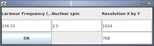
This is the first window which will be displayed.  The larmor frequency in MHz and the nuclear spin can be set in this windows, once O.K. has been selected they can not be changed.  The resolution of the main screen can also be set in this window, the standard setting is usually sufficient, decreasing the resolution is not advised as the text in the program will be cropped.

If a nuclear spin of I=0.5 is used the program will actually set the spin to 2.5, however, it will automatically set the line type to CSA (which is unaffected by the spin of the nucleus) as CSA and kroniker are the only line types which are valid for I=0.5.

If a half integer spin is used, for example I=2.5, the program will start with normal operation.

If an integer spin is used, for example I=1, the program will start and advise you to change the line type.  The line types that are valid are Static, CSA, Kroniker and CSA+Quadrupolar.

Note:-

On some systems the initial window does not appear the correct size, or it apears empty, to solve this problem simply resize the window.  The reason for this occuring is not clear, and I expect it is a problem with Java itself. 

Formatting Input Data

Input data needs to be in one of two different formats, the first is a format which is output by TOPSPIN or a two column data format.  The two formats and to get them are described below.

TOPSPIN 

To gain the format once your data has been processed goto "File", "Save", select the box "Save data of currently displayed region in a text file", click "OK".  In the next box put the save name in the top box, the directory where you would like to save it to in the middle box and "no" in the bottom box.  If you put yes in this box QuadFit will not read the file.   Once this is done the file can be loaded into QuadFit.  If you have zoomed in in Topspin and there is not a even number of points in the output file it will not load in QuadFit.  To circumvent this, remove one point from the end of the file and reduce the number of points as stated at the top of the file by 1.

Two Column Format

This is a format which we have a macro to generate in spinsight.  It is also relatively easy to generate in a spread sheet.  Through my experience I find the Excel tends to put extra information in a text file without telling you.  My personal preference is a spreadsheet program call Gnumeric which is freely available from here.  The format is two colums of data separated with two spaces, the first column is shifts in ppm and the second is corresponding intensities.  The data should be from high shift to low shift, only one data pair per line and an even number of data points.

Notes

Please note that QuadFit can sometimes run into problems if the shifts and intensities are too large, this is particularly unusual and will normally only occur if 0ppm is set at 0MHz.

This program is constantly under development and if you would like to have a file format included please contact me and if I have time and am able to I will include it.

There must be an even number of points in the input file.  If there is an odd number of points then the spectrum will not load in QuadFit.  The extra point can be removed manually from the input file to get around this.

 

Standard Line Shapes (Half integer spin)

For this example we are going to use the default input settings (Larmour Frequency = 156.33MHz, I=2.5) for fitting a ²⁷Al spectra of YAG at 14.1T.

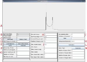Start the program and the initial window will apear (shown above).  Click "OK" and the main window will apear (shown left).

If you wish to follow this example please download the spectra from above.

Click "Load Spectra" and a dialogue box will open which you can then use to browse to the spectra you wish to load.  Select the spectra you wish to load and click "open".  The spectra should then apear in the main window (Panel A).

You should be able to see a red line which is the spectra, the peak in the center of the panel A is the AlO₆ site of YAG and as such has a quadrupole interaction of zero.  On the left hand edge the edge of the AlO₄ site can be seen.  The first thing to do is to make it so the central two lines are visible.  To do this change the "LH Freq (KHz)"  (Panel B) number to 15 and press Return or click "Calculate".  You should now be able to see both the AlO₄ and AlO₆ sites.

Next you can see that the baseline of the spectra and the black line are not aligned, the black line is the total fit and currently looks to be zero (is just very small compared to the spectra).  To correct this DC offset change the number is "Shift Spectra Vertically" to 1500000 and press Return or click "Calculate".  You can change this number as you like to see the effect, it only shifts the spectra vertically.

After every change you must click "Calculate" or press Return, I will now omit this from the rest of the tuition.

Now that we can see the whole spectra we need to increase the size of the simulation.  To do this put 100000000 into the box labeled "Intensity of Line" on panel F.  The shift needs to be corrected next which can be done by putting the number 75 into "Shift of Line (ppm)" on panel F.  Once these values have been input the quality of the simulation is not particularly good and the shift and intensity of the line isn't correct either.

Add some broadening by adding 100 to "Broadening (Hz)" in panel J.  The intensity of the line has dropped which can be corrected later.

The quality of the spectra has now improved, the spectra needs to be fitted more closely however.  To do this use the keyboard short cuts, H for height or "Intensity of Line", S for shift or "Shift of Line (ppm)" and B for broadening.  The other keys required are shift and control.  Shift works to reduce the size of the step and control works to reverse the direction of change.  For example, B increases the broadening, shift+B increases the broadening by a small amount, control+B reduces the amount of broadening and control+shift+B reduces the amount of broadening by a small amount.  When using the key shortcuts care must be taken that none of the text boxes are selected, this can be done by clicking on "Calculate"

As you will notice from my fit the right hand singularity for that site is not a very good fit.  To correct this the Cq of the site needs to be adjusted, this can be done by changing the value in "Min. Quad. Coup." or using the key U in the same manor as H,S and B.

Now to fit the AlO₆ peak.  First add a new line by clicking on "Add Peak" and a second unbroadened peak with the same parameters appears and the number in "Peak Select" changes to 4.

The first thing to do is click on "MAS" in section J until this changes to "kroniker",  then click calculate.  The line will appear to vanish, however it is only small. To correct this change the number in "Intensity of Line" to 100 times it's current value and the line will appear.  Now change the shift until the line lines up with the AlO₆ site either by changing the number in "Shift of Line (ppm)" or by using, Ctrl, Shift and "S".  Change the broadening, height and shift until it fits.

You can then save the final fit by clickinf on "Save" in panel E.  This saves the spectra, total fit, difference and individual lines to the location of your choice.  Remember to write down the parameters used as QuadFit currently doesn't save these. 

 

Distribution of interaction parameters

 Now that the basics have been covered we will produce a distribution in first Cq, then eta and finally both Cq and Eta.

 First start the program with the desired Larmor frequency and  nuclear spin.  Please note that the spin must be greater than 0.5 for this to work and preferably be a half integer to work as this example.

In panel "I" set the minimum quadrupolar coupling constant to 0.1, the maximum coupling constant to 10 and the number of quadrupolar distribution calculations to 100.  The minimum quadrupolar coupling constant should not be set to 0 as this produces a large intensity spike at 0ppm.

 When calculate is depressed the progress bar in the bottom left hand corner will show how much of the calculation is complete and when it reaches 100% the line shape calculated will be displayed.  In this situation there is no line shapes displayed.  This is due to the program not knowing what to display as the values in Panel "M" are asking for a gaussian distribution centred on 0 with a width of 0.

Input the desired centre and width of the gaussian distribution.  In this case we have only calculated a set of lines with varying Cq, and such only a distribution in Cq is meaningful.  A good start value is a centre of 5 and a width of 1.

From this point adjust the centre and width of the distribution, the range over which the lines are calculated is 0.1MHz to 10MHz so when the centre+width and centre-width gets close to these values the line shape will no loger be representative of the real line shape as part of the distribution is artificially truncated.

For a change in the centre and width the change in the line shape is almost instantaneous, however, if you wish to change the range over which the calculation is conducted, the quality of the line calculated or the asymmetry of the line shape then the whole calculation process starts again.

From this stage you should have the basic skills to use the program and as such should  probably play with it for a while to get a feel of how the program works.  If you feel that anything is missing from this tutoral please don't hesistate to contact me.