Hoe Seung Kwon^[1], Department of Economics, University of Warwick

Abstract

An excess co-movement occurs when commodity prices move together even after accounting for the effects of macroeconomic shocks. This article investigates whether fine wine prices co-move excessively with other commodity prices. As one of few articles that investigate wine as a financial diversifier in relation to other commodities, the article extends previous literature by utilising industry-specific production levels and macroeconomic controls from July 2001 to December 2012. Initially, diagonal tests of error terms from OLS and GARCH price models indicate that there may be some interaction between wine and commodity prices. However, vector autoregression and cointegration analysis shows that there is no excess co-movement between fine wine and other commodity prices in either short or long term, strengthening fine wine's status as a financial asset

Keywords: Commodities, fine wine, price movements, VECM, GARCH, excess co-movement

Introduction

With rising income levels, public interest and demand, the global wine trade has increased rapidly over the past decade. The Liv-ex exchange was formed in 1999 to provide an online platform to match the greater consumption and interest in investment-grade wine and to facilitate the trading of wines as financial assets. Alongside other tangible assets such as silver, gold and art (referred to by Roseman (2012) as the SWAG), wine was suggested as a sound alternative investment to diversify and balance a financial portfolio, especially as equities retreated and bond yields tumbled to record lows.

However, apart from the obvious disadvantages of storage costs, fraud and the absence of dividends, some suspect that fine wine prices simply follow the prices of other commodities. As a financial asset, fine wine is sensitive to macroeconomic shocks just like other commodities. Therefore, 'co-movement' of commodity prices comes as no surprise because macroeconomic shocks have similar effects on various commodities. However, if prices still move together after accounting for macroeconomic factors (leaving behind only market fundamentals or a product's unique supply and demand factors), it could imply that 'traders are bullish or bearish on all commodities for no plausible economic reason' (Pindyck and Rotemberg, 1990: 1173) or that there is an 'excess co-movement' (ECM) of commodities.

In particular, Cevik and Sedik (2011: 15) and Bouri (2013: 48) claim that fine wine prices are heavily correlated with oil price. These papers have been reported in various mass media such as the Financial Times, the Economist and the Wall Street Journal to dampen the prospect of wine prices. If true, this poses a detrimental problem for wine as a financial asset because hedgers who want to protect their position by diversifying from commodities can no longer view wine as an alternative investment but as just an extension of oil 'derivatives'. This conclusion seems unusual as, with the advances in econometric techniques, most research has concluded that commodities do not usually exhibit excess co-movement.

Therefore, the principal object of this article is to determine whether wine prices co-move excessively with other commodity prices. This could be further separated into long-run and short-run forms.

Hypothesis 1: After accounting for the effects of macroeconomic shocks, wine prices do not co-move with other commodity prices in the short run.

Hypothesis 2: After accounting for the effects of macroeconomic shocks, wine prices do not co-move with other commodities in the long-run.

Literature review

Previous literature had mainly been aimed towards the establishment of ECM between different commodities. As wine has only recently become a viable financial asset, there is almost no literature analysing wine as a financial diversifier. Consequently, the literature review will firstly evaluate previous work on ECM between other commodities. It will then review a recent paper that has compared wine and oil prices and conclude with this article's contribution to literature.

Initial Modelling of ECM

Even before significant studies on ECM of different commodities, traders had already suspected that there might be a persistent tendency for prices of raw materials to move together (Deb et al., 1996: 275). For example, during the 1973 Oil Shock, prices of sugar, wheat and cocoa rose sharply even though it was an oil supply shock.

Academically, Pindyck and Rotemberg (1990) pioneered the investigation into ECM of unrelated commodities by looking at the effects of macroeconomic variables and their latent variables on prices. With the use of Ordinary Least Squares (OLS), Pindyck and Rotemberg created pricing models of commodities (in this case, wheat, cotton, copper, gold, crude lumber and cocoa) with macroeconomic variables. By carrying out joint tests on the covariance of residuals of commodities, they concluded that price changes remain statistically correlated across commodities even with latent variables and conclude that ECM exists. Pindyck and Rotemberg suggested that 'herd behaviour' of traders is behind this phenomenon. However, while Pindyck and Rotemberg's research provides intuitive initial analysis on ECM, Baillie and Myers (1991: 110) have shown that commodity prices contain unit root and non-normal errors. Therefore OLS regressions on commodity prices yield spurious regression and unbounded variance. Ai et al. (2006: 575) make important improvements on the OLS model by including key supply-side factors, such as production and inventory levels, but the issue of unit root and non-normal errors remained unaddressed.

Use of Cointegration Analysis and GARCH Errors

Palaskas and Varangis (1991: 759) therefore rightly question the robustness of Pindyck and Rotemberg's results. To resolve the unit roots problem, they built an error correction model in pairs and attempt to establish cointegration in different commodities. Palaskas and Varangis justify their use of test in pairs rather than a joint test as one very significant pair in a joint test can lead to the incorrect rejection of ECM. After attempting to establish cointegration and error correction models in different commodities, Palaskas and Varangis conclude that there is no ECM. Interestingly, similar to Pindyck and Rotemberg, they find that as they moved from low to higher frequency observations (i.e. annual to monthly), the amount of co-movement attributed to macroeconomic variables increased while the extent of ECM decreased. This implies that while using macroeconomic variables in the context of OLS is flawed, they may still have high explanatory powers when it comes to commodity price models. However the problem of non-normal errors still remained in Palaskas and Varangis's model.

Acknowledging the problem of non-normal errors, Deb et al. (1996: 286) use GARCH models. As GARCH models allow time-varying variances, they can cater non-normal errors in commodity prices. GARCH models agree with Palaskas and Varangis and confirm that there is no evidence of ECM when tests in GARCH framework are applied. Even in small samples, the model had good power.

Modern adaption of previous work

Cevik and Sedik (2011: 10), however, dispute previous research by applying Pindyck and Rotemberg's OLS model into wine and oil. With the use of OLS, Cevik and Sedik conclude that wine prices have been excessively comoving with oil prices in line with Frankel and Rose's (2010) comments on how 'it cannot be a coincidence that almost all commodity prices rose together during much of the past decade'. Although the model has been slightly improved with the introduction of production figures as suggested by Ai et al. (2006: 575), detrimental flaws found in Pindyck and Rotembergcan still be found in their model. The model suffers from serial correlation, non-normal errors and spurious regression as it only uses level-prices without any adjustment. Their use of production figures is also inappropriate as the authors have used global wine production figures to take into account of supply effects. However, the Liv-ex 50 index, fine wine prices used in the article, all come from Bordeaux.^[2] It would be wrong to assume that production increase in, for example, Chilean mass-produced wine could affect prices of fine Bordeaux wines. Therefore, it is likely that the conclusion on the issue of ECM will change when cointegration tests, GARCH models and better data are introduced.

Contributions to the Literature

This article contributes to the ECM literature in three ways. Firstly, this investigation is the first empirical study on the excess co-movement of wine in relation to other commodities using techniques other than the general OLS model used by Cevik and Sedik (2011: 10). Use of GARCH errors, VAR and cointegration analysis on wine prices has not been tested in the literature so far. Therefore, the results of this analysis will then be compared and contrasted against previous findings in the literature. Secondly, the article uses data that is more suitable for examining ECM relationships, in particular with the addition of more accurate production level and relevant macroeconomic data (further explained in data analysis). Lastly, the article discusses the implications of the ECM tests on the wine market specifically, reviewing wine's status as a financial asset with the new test results.

Data analysis and related issues

Outline of Data

This study uses a dataset containing monthly observations of the commodity prices listed on various commodity exchanges from July 2001 to December 2012 (for a full list of variables and their summary statistics, see Appendix 1). The dataset is primarily constructed from the World Bank, Federal Reserve (FRED) and Eurostat. Most importantly, the prices of fine wine have been provided by Liv-ex, the de facto exchange for professional buyers and sellers of fine wine.

While both higher and lower frequency – daily and annual – data were available, it has been decided that monthly data should be used. One could argue that daily frequency should be used as 'herd behaviour' of traders is probably more apparent in higher frequency (Deb et al., 1996: 275). However, monthly data has been chosen as most macroeconomic data, such as industrial production index and inflation rate, are in monthly frequency. As aforementioned, it is crucial to negate the effects of macroeconomic shocks from the residuals and replicating macroeconomic controls to fit daily frequency would seriously affect the power and validity of these variables. The same logic applies to production level data. Due to their nature as agricultural product and derivative, wheat and wine production data can only be annual. They had to be replicated 12 times to fit monthly-frequency, losing some power, and replicating them to fit the daily frequency would undermine their power and validity even further.

Dependent Variables

The dependent variables to be investigated are the spot prices of five unrelated commodities: wine, oil, gold, copper and wheat. The four commodities other than wine have been proven to be 'unrelated' in their industrial uses and through statistical tests by Pindyck and Rotemberg (1990: 1175) and Deb et al. (1996: 281) (for the results of relationship tests, see Appendix 2). Some may argue that as the majority of commodity trading today is done through futures, futures prices should be used instead. However, futures prices converge towards spot prices during the delivery month and futures may provide arbitrage and speculation. As this research models current values of the commodities rather than their expected, it would be much more appropriate to use spot prices.

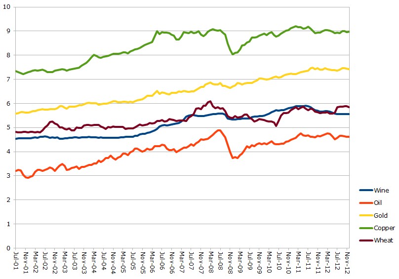
Figure 1: Movements of Logged Commodity Prices

An initial look at the levels data shows that commodities do seem to move very closely with one another. In particular, gold and wine follow very similar pattern and a simple correlation test yields a value of 0.9458 (though this value is highly misleading). Further tests, however, are needed to establish a relationship between the commodities.

Key Explanatory Variables

Production rate

The importance of supply-side factors in constructing a commodity price model is clearly explained in Ai et al. (2006: 575). Unlike other variables, which are in monthly frequency, production rates are set at annual-frequency. This is because, due to the nature of some commodities and lack of information, the only available data were in annual. The same time frame is also used for most other research in the field such as Ai et al. (2006: 577) and Cevik and Sedik (2011: 3). Moreover, a huge improvement has been made on the fine wine production data as it now represents production levels of Bordeaux sub-regions rather than world production levels used in other papers.

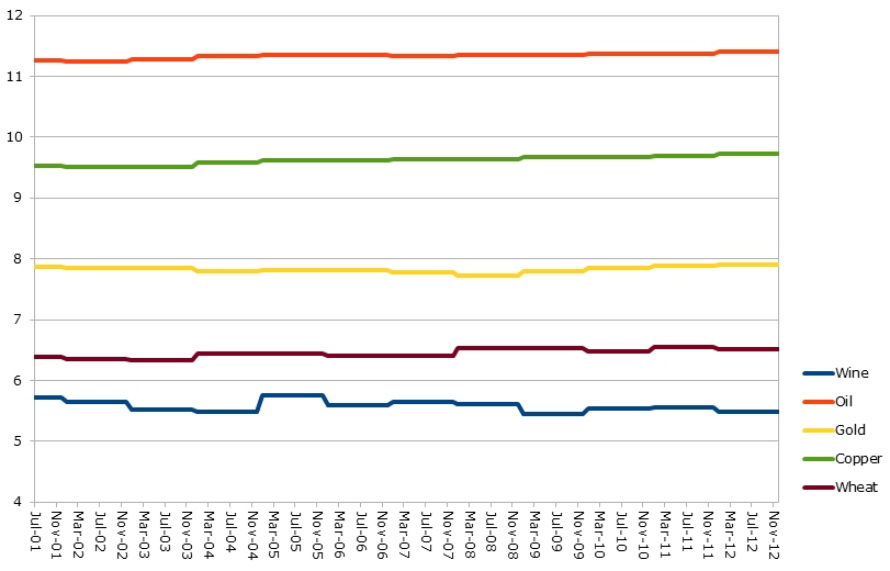
Figure 2: Movements of Logged Commodity Production Levels

The production rates of the commodities have not moved much for all commodities. While the lack of movement is partly due to how data is set at annual frequency, there are legal and technological rationales behind this. Firstly, fine wine is heavily regulated by the European Union and France itself under the Appellation d'Origine Contrôlée system. There is a limit on what kind of grapes can be used, the area of harvest and the maximum yield. Therefore, even if the fine wine producers wanted to increase yield, they would have to go through arduous legal procedures to justify the increase. Moreover, in wine production there is a general trade-off between yield and quality (Matthews and Kriedemann, 2010: 47). As fine wine producers are meticulous about their wine quality, production levels do not change drastically from year to year. Secondly, when it comes to extracting oil, gold and copper it is extremely difficult to suddenly increase production levels due to technological reasons (Renauld et al., 2012:18). While there have been cases where supply of commodities were severely restricted, such as the 1973 Oil Shock, sharp increases requires rare technological breakthroughs. Due to these reasons changes in production rates are very small and one could suspect that they are unlikely to have a great effect on price models/relationships.

Macroeconomic Controls

As accounting for macroeconomic shocks is critical for the investigation, many macroeconomic controls have been included. As well as macroeconomic variables used in other papers (interest rate, inflation, S&P 500 Index and exchange rates), this study has also drawn upon the Industrial Production Index (IPI) of the USA, EU and China. This is because many studies have shown that this index accounts for the bulk of variation in national output over the duration of business cycles. Adding these variables would result in a better control for business cycle fluctuations in the macroeconomy. It is also worth mentioning that the Baltic Dry Index is also added as a macroeconomic shock. The Baltic Dry Index reflects the price of moving major raw materials by sea and is a leading indicator for future economic activity. As trading physical commodities inevitably requires shipping rates and is heavily affected by them, it is a valuable addition to the set of macroeconomic controls.

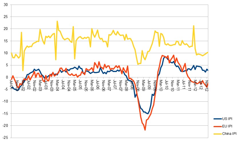
Figure 3: Movement of Macroeconomic Controls

Observing the data reveals that most macroeconomic controls have been reverting at a value with the exception of Industrial Production Index. The sharp changes in the IPIs could heavily affect price models in analysis.

Methodology

Outline of Methodology

Three separate regression techniques will be used to enable an investigation into ECM of wine and other commodities. The analysis will firstly use diagonal tests on covariance of residuals in both OLS and GARCH price models, implement a Vector Autogression (VAR) Model with extensions on Structural VAR Model, and finally test for cointegration between the commodities and its subsequent error correction model.

Motivation for Methodology

Firstly, the Ordinary Least Squares is used to construct price models similar to those of Pindyck and Rotemberg (1990:1177) under the form

ΔPrice = α + β₁ (Production rate) + β₂ (Macroeconomic controls) + β_t (Lags of Price) + ε_t

Lags of variables are only included if there is a clear economic rationale behind the decision and tests for the number of lags agree with the inclusion. Then diagonal tests on the error terms are carried out. A block diagonal structure of the form is hypothesised as

where and represent variance or error terms of two price models. The null hypothesis then tests to see if there is covariance between the two errors. Non-rejection of the null means that the two errors are interacting and there may be ECM.

While the use of differenced models in OLS limit serial correlation issues, the models still suffer from non-normal errors. To solve this, GARCH errors are used. To use GARCH errors, price models are reformulated to reflect GARCH (1,1) structure as below:

P_t = b₀ + b₁P_t-1 + b₂P_t-2 + b₃P_t-3

ε_t - NN(0,h_t) where h_t = α₀ +α₁ε_t-1 + β₁h_t-1

Then the same diagonal tests on the covariance of different commodity price models are executed.

Secondly, VAR model is used to observe any short-run relationship and co-movement between wine and other variables. This is possible as VAR models capture linear interdependencies between two variables. The model will take the form

ΔP_wine,t = α(P_wine,t-1 - KP_{commodity,t-1}) + lagged P_wine + lagged (ΔP_wine, ΔP_commodity) + current and lagged Macroeconomic Variables + production figures of wine and commodity + ε_t

As VAR contains a large number of parameters interacting with one another, it is impractical to interpret the coefficients in the model. Therefore, Impulse Response Functions (IRF), where wine acts as a response and other commodities as impulses, will be used to observe how other commodities may affect wine prices. This is because IRFs can trace the time path of each variable to a one-unit one-time increase (i.e. impulses) to the relevant VAR error. As an extension, a structural VAR model is used so that only commodities affect wine, not the other way round, as some scholars claim that other commodities are driving wine prices. This means setting up matrices so that this view is reflected into VAR models.

Finally, cointegration test and error correction models are used to test for a long-run/error correcting relationship between two commodities. Both Engle-Granger and Johansen tests (for the theory behind the tests, see Appendix 3) will be used to test for cointegrating relationship between the commodities. If such relationship exists then a vector error correction (VECM) model can be formed as below:

ΔP_wine,t = α(P_wine,t-1 - KP_{commodity,t-1}) + β(P_commodity,t - P_{commodity,t-1}) + lagged P_wine + lagged (ΔP_wine, ΔP_commodity) + current and lagged Macroeconomic Variables + lagged production figures of wine and commodity + ε_t

Where ε_t represents the stationary error term and β represents the cointegrating relationship. If there are no cointegrating relationships between the commodities then it could be concluded that there are no long-run ECM.

Empirical results and discussion

Results from diagonal tests between the error terms

Table 1 reports the OLS regression results for initial price models similar to those of Pindyck and Rotemberg (1991: 1177) and Cevik and Sedik (2011: 10). The price models equate to differenced commodity prices to resolve the serial correlation in the models.

	Wine	Oil	Gold	Copper	Wheat
Production Level	-0.0150 (0.0361)	-0.5775 (0.5612)	0.0905 (0.1356)	0.0038 (0.3502)	-0.1653 (0.2156)
US Industrial Production Index	-0.0016 (0.0011)	0.0062* (0.0034)	-0.0017 (0.0018)	0.0035 (0.0031)	0.0039 (0.0030)
China Industrial Production Index	0.0025*** (0.0009)	0.0029 (0.0027)	0.0019 (0.0013)	0.0056*** (0.0024)	-0.0001 (0.0023)
EU Industrial Production Index	0.0019** (0.0009)	-0.0048* (0.0027)	0.0010 (0.0014)	-0.0036 (0.0026)	-0.0004 (0.0024)
Baltic Dry Index	-0.0019 (0.0047)	0.0290* (0.0167)	-0.0028 (0.0082)	0.0157 (0.0151)	-0.0005 (0.0144)
Interest Rates	0.0063*** (0.0024)	-0.0067 (0.0070)	0.0032 (0.0034)	0.0006 (0.0063)	0.0057 (0.0061)
S&P 500	0.0255 (0.0257)	0.1555* (0.0789)	-0.0135 (0.0389)	0.0818 (0.0717)	0.0343 (0.0684)
Exchange Rate Index	-0.0120 (0.0302)	-0.0274 (0.2087)	-0.0388 (0.1030)	0.1913 (0.1896)	-0.0709 (0.1810)
Inflation	-0.0094*** (0.0022)	-0.0136** (0.0066)	-0.0026 (0.0032)	-0.0171*** (0.0059)	-0.0157*** (0.0057)
Constant	-0.0443 (0.3383)	5.3537 (7.3112)	-0.4318 (1.1028)	-1.1750 (4.1754)	1.1761 (1.9977)
R2	0.3077	0.1435	0.0371	0.1432	0.1174

Table 1: OLS Regressions of Differenced Commodities
***, **, * correspond to the coefficient being significant at the 1%, 5% and 10% significance levels respectively

While it is not the central theme of this research, it is interesting to observe that macroeconomic controls have either small or insignificant coefficients on the price of their respective commodities. This could indicate that the effect of macroeconomic shocks on commodities are smaller than economists believe them to be. Unlike macroeconomic controls, however, supply-side factors have much bigger effects on some commodities such as Oil. A 1% percentage increase in oil production levels equate to roughly 0.57% decrease in its price. This makes logical sense as several studies have shown that oil is very sensitive to changes in their price levels (Timilsina et al., 2011: 3; Rockoff, 1984: 613). However, as most coefficients are statistically insignificant and diagonal tests concern error terms from regressions rather than coefficients, there is no need to analyse the coefficients in detail.

	Errors from OLS Regressions			Errors from GARCH Regressions
	R2	Adjusted χ² Value	Prob(χ²)	Adjusted χ² Value	Prob(χ²)
Wine	0.3077
Wine-Oil	0.1435	10.15	0.0014	13.45	0.0002
Wine-Gold	0.0623	0.14	0.7085	0.48	0.4898
Wine-Copper	0.1434	24.31	0.0000	31.04	0.0000
Wine-Wheat	0.1245	0.22	0.6356	3.32	0.0684

Table 2: Diagonal Test between Residuals of OLS Price Model

The diagonal test between the residuals of the OLS price models from Table 2 indicates that the error terms are not identical between Wine-Oil and Wine-Copper relationship. However, for Wine-Gold and Wine-Wheat, the test shows that one cannot reject the null hypothesis of identical error terms. This consequently implies that the error processes of the two models are interacting with one another as Pindyck and Rotemberg (1990: 1173) suggested.

To take the tests even further, price models are reformulated under the GARCH(1,1) form (the results of price models are in Appendix 4) as Skewness/Kurtosis, Shapiro-Francia and Shapiro-Wilk tests have shown that the errors in prices are non-normal as expected (the test results are in Appendix 5). However, even accounting for the fact that the error terms in differenced price models are non-normal with GARCH error terms, the relationship between Wine-Gold still remains (Table 2). The results of diagonal tests on the errors could therefore imply that wine and gold prices are excessively commoving to some extent.

However, the covariance and consequently correlation between the errors only merely exhibit that the two models' error processes are interacting to some extent. Whether one follows with one another needs to be tested using other methods.

Results from VAR models and structural VAR

After testing for how many lags to add in VAR regressions using information criteria (for the results, see Appendix 6), VAR regressions were completed with macroeconomic controls as exogenous variables (full results of the VAR regressions are in Appendix 7). Again commodity prices were differenced because VAR models require all variables to be of the same order of integration. As mentioned in the data analysis, rather than interpreting coefficients of VAR regressions directly, Impulse Response Functions, where impulses are other commodities and the response is 'wine', are used instead.

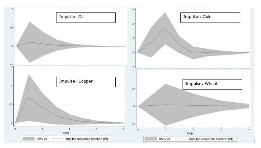
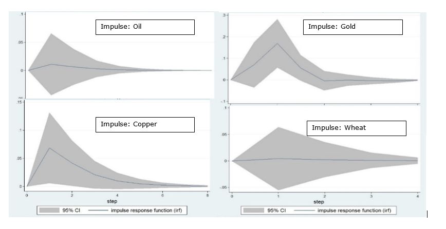
Figure 4: Impulse Response Function where Response: Wine Prices

The IRFs report that there may be very short-term effects of a change in commodity prices of wine. This is most evident from the impulses of gold and copper. It is also worth noting that all the impulses result in positive movement of wine prices up to 1 or 2 months. However, IRFs resort back to 0-value indicating that there are no long-term effects of changes in commodity prices on wine. The responses are also within the confidence interval range at 0-value, meaning that IRFs do not indicate a definitive short-run effect on wine. One can be confident about the conclusions of IRFs, as underlying VAR models were stationary and stable according to the eigenvalue test (the results of the tests are in Appendix 9). However, the forecasting power of the models were weak even for in-sample forecasting as the models were not dynamic. To test the hypothesis even further, a structural VAR model is created where only other commodity prices interact with wine prices but not the other way round. However, the IRFs of the structural VAR yielded identical results (Results in Appendix 8)

Results of Cointegration Tests

To test if there are any long-term relationships between wine and other commodities, an investigation on cointegrating relationships can be used. As expected from Baillie and Myers (1991:110), unit root tests through Augmented Dickey Fuller (ADF) test, Philip-Perron test and GLS-transformed ADF test confirm that all the commodity prices exhibited unit roots (the test results are in Appendix 10). Here, the prices are not differenced as setting up a cointegrating relationship requires two or more equations containing unit roots. After confirming the existence of unit roots, two tests to identify the number of cointegrating relationships can be carried out.

Johansen Test

	Suggested Rank	Trace Statistic	5% Critical Value
Wine			15.41
Wine-Oil	0	7.5507	15.41
Wine-Gold	0	4.0844	15.41
Wine-Copper	0	11.0561	15.41
Wine-Wheat	0	14.9337	15.41

Table 3a: Results of cointegration tests

Engle-Granger Test in the form of a unit test on error of cointegrating regression

Cointegrating relationship	Augmented Dickey Fuller	5% Mackinnon Critical Value
Wine-Oil	-1.632	-2.862
Wine-Gold	-1.174	-2.862
Wine-Copper	-1.205	-2.862
Wine-Wheat	-2.079	-2.862

Table 3b: Results of cointegration tests

Cointegrating relationship	GLS-transformed Augmented Dickey Fuller	Max Number of Lags from Schwert Criterion	5% Critical Value
Wine-Oil	-1.506	13	-2.774
Wine-Gold	-2.560	13	-2.774
Wine-Copper	-1.458	13	-2.774
Wine-Wheat	-1.741	13	-2.774

Table 3c: Results of cointegration tests

Both test methods reveal that wine does not have a long-term cointegrating relationship with other commodities. This is identical to the conclusion from IRF analysis as all the impulses failed to make any long-term effects on wine prices. Consequently, one cannot form an error correction model between wine and other commodities. Various specifications of the estimates were tested, such as different number of lags on the Johansen test, but results remained identical with a cointegrating rank of zero. Moreover, a GLS-transformed ADF test was introduced to challenge the hypothesis as rigorously as possible but again this did not affect the lack of a cointegrating relationship. Palaskas and Varangis (1991: 29), who use the same Engle-Granger test for other commodities also find no significant cointegrating relationships.

Conclusion and evaluation

Conclusion

This article set out to investigate whether wine prices are 'comoving excessively' with other commodity prices. Using data from July 2001 to December 2012, we find that there is no ECM between fine wine prices and other commodity prices. While one could observe some interactions between the error terms of price models in both OLS and GARCH error terms, this did not translate to any short-term or long-term relationships as examined through VAR and cointegration tests.

One reason could be that the 'herd behaviour', which is usually the reason given by other research papers as the cause of ECM (Pindyck and Rotemberg, 1990 in particular), has not been observed in the commodities market in general. While disregarding herd behaviour and irrational behaviour of traders is beyond the scope of this research, a large amount of literature agrees with this idea (DeMirer et al., 2013: 2; Steen and Gjolberg, 2012: 80). If herd behaviour was present it would have resulted in an ECM at least in the short term.

Secondly, in commodity markets, market fundamentals that drive prices are much more visible than other markets. For example, the consequences of bad weather and extraction rates on commodity prices can easily be deduced. As the influence of individual market fundamentals are so unique in different commodities, it seems natural that there is no ECM, even though they may briefly move together during macroeconomic shocks. This applies to wine in particular as wine has so many market fundamentals that are unique to itself. As well as production levels, quality of wine, vintage and location are extremely important as price factors.

Policy Implications

Dispelling the myth that wine co-moves with other commodities is an important step in establishing wine as a financial asset. An investable commodity should always give an investor an option to hedge against unforeseen changes. As wine does not excessively co-move with other prices, investors can use wine as a hedge against other financial assets as wine would be independently priced and uninfluenced by factors solely-affecting other commodities. Some literature (Sanning et al., 2008: 52; Jones and Storchmann, 2001: 116) has already concluded that wine has very low exposure to market risk factors, offering a valuable dimension of portfolio diversification.

However, whether the conclusion of this article allows wine to be a full functioning financial asset with extensions such as creation of derivatives, options and futures contracts remains unanswered. Although this has been lifted massively with the introduction of Liv-ex index, the wine market still suffers from product heterogeneity, incomplete information and opacity of valuation rules. Moreover, wine as a product holds great sentimental values to its producers, which can create further market distortions. For example, when the Liv-ex introduced an option to short-sell Lafite 2009 on its index, it caused an 'outrage amongst wine merchants' even though 'this sort of trading would not raise an eyebrow outside wine trade' (Lechmere, 2010: 29). The wine market therefore needs to overcome these issues to become a much more widely accepted financial asset.

Limitations of the Project

The limitations concerning this article mainly come from the data itself. Firstly, the data may suffer from small sample bias. While 138 samples are enough to carry out ample economic analysis, this is still substantially less than those of other research. Other research typically tracks commodities prices for more than two decades. The lower number of observations is due to the fact that the wine price index is till at an infancy stage and has only been around for the last decade or so. Therefore, giving the index more time and analysing ECM at a later date would further increase the validity of research.

Secondly, even though this article has justified the use of monthly frequency data for the aims of this study, it should be noted that if herd behaviour was present and caused ECM, it is more likely to appear in higher-frequency data. Consequently, the investigation is unlikely to detect any intra-day or daily ECM of wine and other commodities. This underestimates the presence of ECM and results in a negative bias, reducing the validity of the results.

Potential Extensions

A sizeable improvement could be made on the investigation with the use of stock and inventory levels. While the trading of commodities has been driven by futures contracts over the past decades, trade of physicals are heavily affected by stock and inventory levels of commodities (Roache and Erbil, 2010). Therefore, it could be argued that inventory levels are just as important as fundamental demand when it comes to pricing the commodities. For example, Hieronymus (1977: 149) explains that prices may be at a discount when there is a lack of warehouse space and are tied to the cost of putting commodity into storage.

Unfortunately, there is almost no data on inventory levels regarding wine and even for other commodities, inventory data is regarded as specialist knowledge. As well as the discreet nature of data, there is the problem of fraud and counterfeit goods as wine is a luxury consumable good as well as a financial instrument. For example, in China alone, it is often said that there are 10 times more bottles labelled 'Chateau Latour' wine than the whole annual production levels of the Chateau. The addition of the variables would contribute greatly towards the research but it would be difficult to collect the figures.

The scope of this research could be extended from the commodities market to the wider financial market to see whether wine can act as a hedge against other financial assets such equities and bonds.

---

List of figures

Figure 1: Movement of Logged Commodity Prices

Figure 2: Movement of Logged Commodity Production Levels

Figure 3: Movement of Macroeconomic Controls

Figure 4: Impulse Response Function where Response: Wine Prices

List of tables

Table 1: OLS Regressions of Differenced Commodities

Table 2: Diagonal Test between Residuals of OLS Price Model

Table 3: Results of cointegration tests

Appendices

Appendix 1: Descriptions of Variables Used in the Analysis

*Variables are in Natural Logarithm with the exception of interest, inflation, usipi, euipi and chipi

Variable	Frequency	Source	Explanation
lwine	Monthly	Liv-ex Exchange	Price of Liv-ex 100 Index (tracks the movement of 100 most sought-after fine wines (Liv-ex))
loil	Monthly	World Bank	Spot Price of West Texas Intermediate FOB in USD per Barrel (NYMEX)
lgold	Monthly	World Bank	Spot Price of 99.5% Gold (UK) afternoon fixing USD per Troy Ounce (COMEX)
lcopper	Monthly	World Bank	Spot Price of Copper, Grade A Cathode, USD per metric ton (LME)
lwheat	Monthly	World Bank	Spot Price of Wheat, No.1 Hard Red Winter FOB, at USD per metric ton (COMEX)
interest	Monthly	Federal Reserve	US 3 Month-Bill Treasury Rate
inflation	Monthly	US Bureau of Labor Statistics	Monthly Inflation rate based on annual change on US Consumer Price Index
sp500	Monthly	Bloomberg	S&P 500: Stock Market Index based on market capitalizations of 500 large companies on NYSE
exchange	Monthly	Federal Reserve	Trade-Weighted Effective Exchange Rate Index of USD
usipi	Monthly	Federal Reserve	Monthly changes in US Industrial Production Index
euipi	Monthly	Eurostat	Monthly changes in EU Industrial Production Index
chipi	Monthly	National Bureau of Statistics of China	Monthly changes in Chinese Industrial Production Index
lbdi	Monthly	Baltic Exchange	Baltic Dry Index: assessment of price of moving major raw materials by sea covering 23 shipping routes on a time charter basis
pwine	Annual	France Agrimer	Production estimate of wine in Pauillac, Margaux, Leognan regions in 1000 Hectolitre
poil	Annual	US Energy Information Administration	Global production estimate of crude oil in Thousand Barrels Per Day
pgold	Annual	US Geological Survey	Global production estimate of gold in metric tons
pcopper	Annual	US Geological Survey	Global production estimate of copper ores in thousand metric tons
pwheat	Annual	Food and Agricultural Organisation (UN)	Global production estimate of wheat in million metric tons

Summary Statistics of Variables

Variable	Number of Observations	Mean	Standard Deviation	Minimum	Maximum
lwine	138	5.1388	0.48421	4.5249	5.8990
loil	138	4.0357	0.52781	2.9188	4.8869
lgold	138	6.5235	0.58790	5.5892	7.4792
lcopper	138	8.3998	0.64208	7.2279	9.1983
lwheat	138	5.3280	0.34302	4.7995	6.0861
interest	138	1.7069	01.7045	0.0100	5.1600
inflation	138	2.4166	01.3919	-2.1000	5.6000
sp500	138	7.0634	0.15950	6.6295	7.3393
exchange	138	4.4111	0.13014	4.2344	4.7202
usipi	138	.65463	4.9343	-15.0200	8.5000
euipi	138	.17681	5.9950	-21.8000	9.1000
chipi	138	14.2210	3.7347	2.7000	23.2000
lbdi	138	7.8051	0.72230	6.5221	9.3448
pwine	138	5.5797	0.09142	5.4424	5.7621
poil	138	11.3375	0.04280	11.2524	11.4005
pgold	138	7.8256	0.04891	7.7231	7.9011
pcopper	138	9.6232	0.06494	9.5178	9.7232
pwheat	138	6.4513	0.07185	6.3284	6.5569

Appendix 2: 'Unrelated' relationship tests

Examining whether the commodities in question are unrelated is important as ECM is intended to apply to commodities that are unrelated through joint production or consumption. To examine whether the commodities are unrelated, Pindyck and Rotemberg (1990) carried out a likelihood ratio test of the hypothesis that the correlation matrix is equal to the identity matrix where the ratio of restricted and unrestricted likelihood function is λ = |R|^N/2 where |R| is the determinant of the correlation matrix.

The test statistics is consequently -2 logλ which is distributed as χ² with (I/2) p(p-I) degrees of freedom, where p is the number of commodities. This equates to a test statistic of 114.6 and individual correlation statistics that exceed 0.112 in magnitude are significant at 5% level.

Correlations of Monthly Log Changes in Commodity Prices

	Oil	Gold	Copper
Gold	0.245	-	-
Copper	0.032	0.322	-
Wheat	0.103	-0.020	0.051

From the correlation of monthly log changes in commodity prices, one can observe that gold may be 'related' with oil and copper. However, when Deb, Trivedi and Varangis (1996) use the similar test on data from 1974, they find that only Gold and Copper are related due to their joint consumption as metallic alloys. However, when putting the analysis into the context of wine, the two commodities, Gold and copper yields no correlation and is 'unrelated' as they do not share any joint consumption nor production. Therefore it would be safe to assume that the four commodities in question – oil, gold, copper and wheat – are unrelated to wine.

Appendix 3: Theory behind Engle-Granger test and Johansen test

Engle-Granger Test (Palaskas and Varangis, 1991)

Assume that there is a hypothesised relationship between two prices in the following form

Y_t - KX_t = Z_t

where Y_t and X_t represent natural logarithms of two commodity prices, Z_t represents any short-run deviation from their long-run relationship. For Y_t and X_t to be cointegrated, Z_t must be a stationary process i.e. reject the hypothesis of unit roots.

Johansen Test (Johansen, 1991)

The null hypothesis of the test is that there are no more than r cointegrating relationships. Johansen represents the trace statistic as

Where T is the number of observations and are estimated eigenvalues. This is based on Johansen's maximum likelihood estimators of the parameters of a cointegrating VECM where the basic VECM is

Where y is a (K x 1) vector of I(1) variables, and are (K x r) parameter matrices with rank r<K, are (K x K) matrices of parameters and ε_t is a (K x 1) vector of normally distributed errors that is serially uncorrelated by has contemporaneous covariance matrix Ω.

Appendix 4: Price Models in the form GARCH(1,1)

For the regression results below, the price models of commodities are in GARCH(1,1) form

P_t = b₀ + b₁P_t-1 + b₂P_t-2 + b₃P_t-3

ε_t - NN(0,h_t) where h_t = α₀ +α₁ε_t-1 + β₁h_t-1

	Wine	Oil	Gold	Copper	Wheat
LM-Test for ARCH effect	0.0775	0.0000	0.1858	0.0000	0.0285
Constant of variable itself	0.0068*** (0.0015)	0.0207*** (0.0071)	0.0132*** (0.0035)	0.0159*** (0.0058)	0.0038 (0.0062)
ARCH parameter	1.0308*** (0.1568)	0.3693*** (0.1392)	0.1562 (0.0968)	0.4688*** (0.1272)	0.3216*** (0.1358)
GARCH parameter	-0.0040 (0.0792)	-0.0691 (0.2185)	0.6430*** (0.2429)	0.2730 (0.1911)	0.4642*** (0.1959)
Constant	0.0002*** (0.0001)	0.0045*** (0.0012)	0.0003 (0.0002)	0.0017*** (0.0006)	0.0013 (0.0006)

***, **, * correspond to the coefficient being significant at the 1%, 5% and 10% significance levels respectively

While the Lagrange Multiplier Test indicates that there are no ARCH effects in Oil and Copper, price models were reformulated to reflect non-normal errors in commodity prices. As the article focuses on the error terms of these models, there are no direct implications of the coefficients of ARCH and GARCH parameters.

Appendix 5: Normality Tests on the error terms of dependent variables

Skewness/Kurtosis Tests for Normality

Variable	Pr(Skewness)	Pr(Kurtosis)	Adjusted χ² Value	Prob(χ²)
Wine	0.9058	0.0000		0.0000
Oil	0.0535	0.0000	20.59	0.0000
Gold	0.5766	0.0000	65.19	0.0000
Copper	0.0077	0.0000	43.28	0.0000
Wheat	0.1546	0.0000	24.26	0.0000

Shapiro-Francia/ Shapiro-Wilk for Normal Data

Variable	W'	V'	Adjusted Z Value	Prob(Z)
Wine	0.8553	17.2010	5.7420	0.0000
Oil	0.9463	6.3800	3.7400	0.0001
Gold	0.9417	6.9320	3.9080	0.0000
Copper	0.8667	15.8440	5.5760	0.0000
Wheat	0.9534	5.5340	3.4530	0.0003

Shapiro-Wilk W Test for Normal Data

Variable	W	V	Adjusted Z Value	Prob(Z)
Wine	0.8493	16.3200	6.3030	0.0000
Oil	0.9410	6.3870	4.1850	0.0000
Gold	0.9346	7.0830	4.4190	0.0000
Copper	0.8601	15.1480	6.1350	0.0000
Wheat	0.9481	5.6210	3.8970	0.0001

Skewness/Kurtosis Test, Shapiro-Francia and Shapiro-Wilk Test for normality. From the table, one can reject the hypothesis that all the commodities are normally distributed.

Appendix 6: Use of information criteria to decide how many lags should be added to VAR models

Variables in VAR	Suggested Lags	AIC	HQIC	SBIC
Wine-Oil	1	-6.7285	-6.67551*	-6.5981*
Wine-Gold	2	-8.09496*	-8.00665*	-7.87764
Wine-Copper	1	-7.06772*	-7.01473*	-6.93733*
Wine-Wheat	1	-6.87837*	-6.82538*	-6.74798*

* indicates the suggested number of lags equate to the optimal number of lags given by particular information criterion

This table is included to justify the number of lags added to the VAR models. Information Criteria indicated the suggested number of lags for VAR Models with Wine-Oil, Wine-Gold, Wine-Copper and Wine-Wheat are 1, 2, 1 and 1 respectively.

Appendix 7: VAR regressions with exogenous variables (coefficients of exogenous variables not shown)

	Coefficient of parameters
VAR with Wine-Oil
Wine interacting on Wine	0.3723 (0.0872) ***
Oil interacting on Wine	0.0107 (0.0279)
Wine interacting on Oil	0.4892 (0.2779) *
Oil interacting on Oil	0.1971 (0.0891) **
VAR with Wine-Gold
Wine lag 1 interacting on Wine	0.3657 (0.0892) ***
Wine lag 2 interacting on Wine	-0.0176 (0.0891)
Gold lag 1 interacting on Wine	0.0694 (0.0534)
Gold lag 2 interacting on Wine	0.1409 (0.0527) ***
Wine lag 1 interacting on Gold	0.2951 (0.1471) **
Wine lag 2 interacting on Gold	-0.3360 (0.1468) **
Gold lag 1 interacting on Gold	0.0411 (0.0881)
Gold lag 2 interacting on Gold	-0.1801 (0.0870) **
VAR with Wine-Copper
Wine interacting on Wine	0.3037 (0.0902) ***
Copper interacting on Wine	0.0685 (0.0320) **
Copper interacting on Copper	0.4245 (0.2543) *
Wine interacting on Copper	0.3019 (0.0902) ***
VAR with Wine-Wheat
Wine interacting on Wine	0.3805 (0.0843) ***
Wheat interacting on Wine	0.0041 (0.0302)
Wheat interacting on Wheat	-0.2453 (0.2398)
Wine interacting on Wheat	0.1748 (0.0861) **

***, **, * correspond to the coefficient being significant at the 1%, 5% and 10% significance levels respectively

Interpretation of VAR models are completed indirectly through the use of Impulse Response Functions, based on these VAR regressions.

Appendix 8: Structural VAR Regressions

To create VAR models where only other commodities are interacting on wine, not the other way round, one requires two matrices under the form

Matrix A =

Matrix B =

Under the matrices, it is structured so that commodities have coefficient of 1 for interactions with itself. The coefficient of wine interacting with other variables is constrained at 0 while other commodities affecting wine are left for the VAR to estimate.

	Coefficient of parameters
VAR with Wine-Oil
Wine interacting on Wine	1 (constrained)
Oil interacting on Wine	-0.6364 (0.2678)**
Wine interacting on Oil	0 (constrained)
Oil interacting on Oil	1 (constrained)
VAR with Wine-Gold
Wine lag 1 interacting on Wine	1 (constrained)
Wine lag 2 interacting on Wine	1 (constrained)
Gold lag 1 interacting on Wine	0.0531 (0.1418)
Gold lag 2 interacting on Wine	0.0241 (0.0014)
Wine lag 1 interacting on Gold	0 (constrained)
Wine lag 2 interacting on Gold	0 (constrained)
Gold lag 1 interacting on Gold	1 (constrained)
Gold lag 2 interacting on Gold	1 (constrained)
VAR with Wine-Copper
Wine interacting on Wine	1 (constrained)
Copper interacting on Wine	-0.8691 (0.2298)***
Copper interacting on Copper	0 (constrained)
Wine interacting on Copper	1 (constrained)
VAR with Wine-Wheat
Wine interacting on Wine	1 (constrained)
Wheat interacting on Wine	-0.2181 (0.2432)
Wheat interacting on Wheat	0 (constrained)
Wine interacting on Wheat	1 (constrained)

***, **, * correspond to the coefficient being significant at the 1%, 5% and 10% significance levels respectively

While one can observe the differences in the coefficients of unconstrained parameters, IRFs produced from structural VAR models are identical to those of unconstrained VAR models.

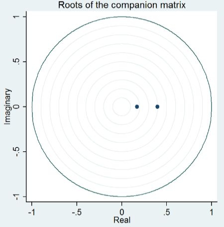
Appendix 9: VAR Stability Tests

The stationarity and stability of VAR Models can be checked using the companion matrix of the models. The companion matrix takes the form

And obtains eigenvalues using matrix eigenvalues. Here the modulus of the complex eigenvalue r+ci is . The VAR Model in question would be stable if the modulus of each eigenvalue is strictly less than 1. Applying the stability test to the 4 VAR models clearly show that the modulus all the eigenvalues are strictly less than 1 as can be seen through companion matrix graphs:

VAR Model with Wine-Oil

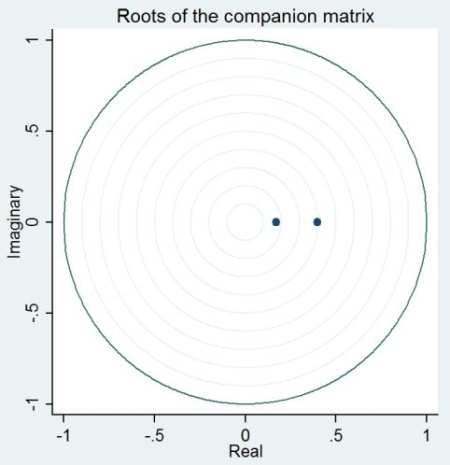
VAR Model with Wine-Gold

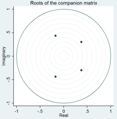
VAR Model with Wine-Copper

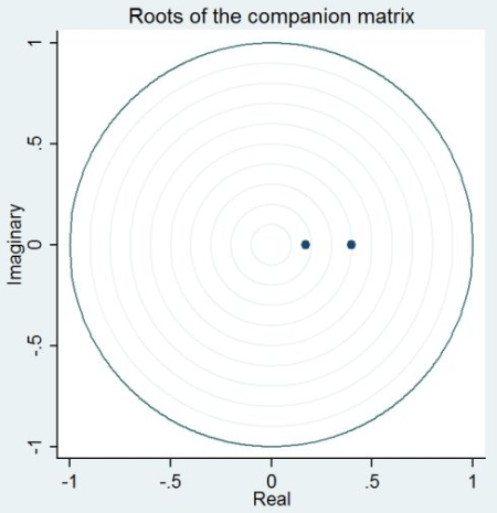
VAR Model with Wine-Wheat

Appendix 10: Unit root test results

Augmented Dickey Fuller Test on the levels of Logged Commodity Prices

	Ideal number of lags from information criteria	Augmented Dickey Fuller Test Statistic	5% Critical Value
Wine	2	-1.051	-2.888
Oil	2	-1.690	-2.888
Gold	1	-0.489	-2.888
Copper	2	-1.710	-2.888
Wheat	2	-1.546	-2.888

GLS-transformed Augmented Dickey Fuller Test on the levels of Logged Commodity Prices

	GLS-transformed Augmented Dickey Fuller	Max Number of Lags from Schwert Criterion	5% Critical Value
Wine	-2.572	13	-2.774
Oil	-1.867	13	-2.774
Gold	-2.151	13	-2.774
Copper	-1.585	13	-2.774
Wheat	-2.286	13	-2.774

As test statistics are larger algebraically than any of the displayed critical values, we do not reject the null hypothesis of a unit root in all the variables.

Notes

[1] Hoe Seung Kwon has completed his undergraduate studies in Economics at the University of Warwick in 2014. He is currently working as a commodity trader in Singapore/Brazil and hopes to continue his interests in commodities, wine and whisky.

[2] More specifically 'fine wine' in the index is made up of last ten vintages of 'Premier Cru' of the 1855 Bordeaux classification which are Château Margaux, Château Lafite, Château Mouton-Rothschild, Château Haut-Brion and Château Latour. They are located in Margaux, Pauillac and Pessac-Leognan, which are sub-regions of Bordeaux.

References

To cite this paper please use the following details: Kwon, H.S. (2014), 'An Investigation into the Excess Co-movement of Fine Wine and Commodity Prices', Reinvention: an International Journal of Undergraduate Research, BCUR 2014 Special Issue, http://www.warwick.ac.uk/reinventionjournal/issues/bcur2014specialissue/kwon/. Date accessed [insert date]. If you cite this article or use it in any teaching or other related activities please let us know by e-mailing us at Reinventionjournal at warwick dot ac dot uk.

References

Ai, C., A. Chatrath and F. Song (2006),' On the Co-movement of Commodity Prices',American Agricultural Economics Association, 88, 574-88
Baillie, R. and R. Myers (1991), 'Bivariate GARCH Estimation of the Optimal Commodity Futures Hedge', Journal of Applied Econometrics, 6, 109-24
Bouri, E. (2013), 'Do Fine Wines Blend with Crude Oil? Seizing the Transmission of Mean and Volatility between Two Commodity Prices', Journal of Wine Economics, 8, 46-68
Cashin, P., C. J. McDermott and A. Scott (1999), 'The Myth of Comoving Commodity Prices', The International Monetary Fund, WP/99/169, 1-20
Cevik, S. and T. Sedik (2011), 'A Barrel of Oil or a Bottle of Wine: How Do Global Growth Dynamics Affect Commodity Prices?', The International Monetary Fund, WP/11/1, 1-20
Deb, P., P. Trivedi and P. Varangis (1996), 'The Excess Co-movement on Commodity Prices Reconsidered', Journal of Applied Econometrics, 11 (3), 275-91
DeMirer, R., H. Lee and D. Lien (2013), 'Commodity Financialization and Herd Behavior in Commodity Futures Markets', The University of Texas Working Paper Series, No.0046
Frankel, J. and Rose, A. (2010), 'Determinants of Agricultural and Mineral Commodity Prices' Harvard University, Scholarly Articles 4450126
Hieronymus, T. (1977), 'Economics of Futures Trading for Commercial and Personal Profit', NY: Commodity Research Bureau Inc. 148-71
Jones, G. and K. Storchmann (2001), 'Wine Market Prices and Investment Under Uncertainty: An Econometric Model for Bordeaux Crus Classes', Agricultural Economics, 26, 115-33
Lechmere, A. (2010), 'Liv-ex Lafite 09 trade causes outrage - and acceptance', Decanter Magazine, June 2010, 29
Matthews, M. and P. Kriedemann (2006), 'Water Deficit, Yield, Berry Size as Factors for Composition and Sensory Attributes of Red Wine', in Proceedings of the Australian society of viticulture and oenology: 'Finishing the Job' - optimal ripening of Cabernet Sauvignon and Shiraz, Mildura: Australian Society of Oenology and Viticulture, pp.47-54
Meloni, G. and J. Swinnen (2013), 'The Political Economy of European Wine Regulations', Journal of Wine Economics, 8 (3), 244-84
Palaskas, T. and P. Varangis (1991), 'Is There Excess Co-Movement of Primary Commodity Prices?', The World Bank, WPS 75
Pindyck, R. and J. Rotemberg (1990), 'The Excess Co-Movement of Commodity Prices', The Economic Journal, 100 (403), 1173-89
Renauld, C., M. Jebrak and J. Vaillancourt (2012), 100 Innovations in the Mining Industry, Quebec: The Mining Association of Canada Press
Roache, S. and N. Erbil (2010), 'How Commodity Price Curves and Inventories React to a Short-Run Scarcity Shock', The International Monetary Fund, WP/10/222
Roseman, J. (2012), SWAG: Alternative Investments for the Coming Decade, Guildford: Grosvenor House Publishing
Rockoff, H. (1984), 'Some Evidence on the Real Price of Gold, Its Cost of Production and Commodity Prices', in Bordo, D. and A. Schwartz (eds), A Retrospective on the Classical Gold Standard, 1821-1931, Chicago: University of Chicago Press, pp. 613-650
Sanning, L., Shaffer S. and J. Sharratt (2008), 'Bordeaux Wine as a Financial Investment', Journal of Wine Economics, 3 (1), 51-71
Steen, M. and O. Gjolberg (2012), 'Are commodity markets characterized by herd behaviour?', Applied Financial Economics, 23 (1), 79-90
Timilsina, G., S. Mevel S. and A. Shrestha (2011), 'World oil price and biofuels: a general equilibrium analysis', Policy Research Working Paper Series 5673, The World Bank, 1-27