A Review of Relay Auto-tuning Methods for the Tuning of PID-type Controllers
Stephen Hornsey[1], School of Science and Engineering, Teesside University
Abstract
This paper considers frequency point identification and PID-type controller tuning through the use of relay feedback methods, based on those originally given by Åström and Hägglund in 1984. The proposed concepts and supporting theory are first explored before more recent developments are investigated. Two methods which aim to increase the accuracy of frequency point identification are studied and applied to a coupled tanks rig, where the benefits are apparent. The focus then turns to using the identified frequency points to arrive at a set of PID-type controller parameters. A number of tuning methods are considered from the simple method first proposed by Åström and Hägglund to more advanced methods for robust design. Pleasing results are seen in application to the coupled tanks rig, especially in the case of a tuning method which gives an 'iso-damping' property. Finally, recommendations are given regarding the situations in which the proposed methods may, or may not, be beneficial.
Keywords: PID control, auto-tuning, limit cycle, relay feedback, frequency response, robustness.
Introduction
The PID-type controller is used in more than 95% of control loops in the process industry (Åström and Hägglund, 1995). A PID-type controller can be very effective in driving a measured process variables, such as level, flow, or temperature to a desired set point. The operating principle of the PID controller is in the measurement of the error between the process variable and the set point. The proportional element gives a controller output depending on the magnitude of this error; integral action serves to eliminate steady-state error, while derivative action works to inhibit rapid changes in the process variable. These three control signals are combined to give a unified control effort. The popularity of the PID controller is due to the fact that it is an easy concept to understand and its performance is, at least, satisfactory for the majority industrial control applications. The transfer function for a parallel algorithm PID controller, as used in this paper is:
where kc is the proportional gain, Td is the derivative-action time, and Ti is the integral-action time.
However, derivative action can often cause undesirable loop performance, for example, a kick in the error signal when a step input is applied. For this reason, in many practical applications the derivative term is placed in the feedback path, hence taking the derivative of the output and resulting in a smoother response.
It is important to understand that efficient performance can only be guaranteed if a given controller has been tuned to suit the specific process on which it is acting. In order to tune a controller to give a desired response, the engineer must select values of proportional, integral and derivative gain. Historically, tuning of control loops has been a subjective, heuristic process, with control engineers relying on existing knowledge of the system and skill. It can often be the case that the tuning process can be very difficult and time consuming.
An insight is given by the paper presented by Bialkowksi (Bialkowski, 1993) which gives details of audits of paper mills in Canada, where it is stated that, of a typical 2000 control loops in a single paper mill, 20% were not working efficiently with 30% of these cases caused by poor or incorrect tuning. Furthermore, a separate survey by Ender (Ender, 1993) gives similar conclusions, stating that 30% of the studied controllers operated in manual mode and 20% of control loops use the tuning with which they were supplied from the factory. In an industrial process setting the maximisation of profit is paramount. A way in which profit can be maximised is through the optimisation of the process itself by ensuring throughput is as close as possible to upper limits for the highest possible amount of time. For this to be realised, tight control over systems is necessary. Therefore, it is beneficial to have available a tuning strategy which will give good results, without the need for subjective decision making, and which can be achieved quickly.
Today, there are many methods available for the tuning of PID controllers. Examples are: direct pole placement, internal model control (Garcia and Morari, 1982) and optimisation based methods, such as that given by Argelaguet (Argelaguet, 1996). Here focus will be made on those methods concerning frequency response, where knowledge of the system's response to specific frequencies is employed.
During past decades, many simple frequency response-based tuning rules have been presented with the intention of allowing the engineer to select suitable values for the PID parameters easily. Examples include the no overshoot rule (Seborg, Edgar and Mellichamp, 1989), some overshoot rule (Seborg, Edgar and Mellichamp, 1989), Pessen integral rule (Pessen, 1994), Ziegler-Nichols rule (Nichols and Zeigler, 1942) and refined Ziegler-Nichols rule (Hang, Åström and Ho, 1991). Each of these rules uses measured values referred to as the ultimate gain and period of a given process to give a set of PID controller parameters. In simple terms, the ultimate gain and period of a system are related to the steady oscillation or limit cycle which is produced when the system is pushed to the limit of stability with an increase in loop gain. However, the ultimate gain and period provide only a limited insight into the behaviour of the process in question, and so it is often the case that the closed loop response is less than satisfactory. One such example is that the Ziegler-Nichols tuning rule is optimised to give a good disturbance response but typically gives a poor response to a change in set point. Further problems can be encountered if the characteristics of the system tend to vary with time.
Because these rigid controller tuning rules are often not sufficient, a number of methods which are able to provide automatic and adaptive tuning to changing process characteristics have been developed. These include pattern recognition (Bristol, 1977), relay auto tuning (Åström and Hägglund, 1984a), and stepwise parameter optimisation (Radke and Isermann, 1987). These methods are based on the automatic measurement of the ultimate gain and period, and are useful where little is known about the process characteristics and there is variation in process dynamics. It is the relay auto tuning method that is considered in this paper.
Relay Auto-Tuning
In recent years, a number of automated relay tuning methods have been developed. One of the most notable is the Åström-Hägglund method as presented in 1984 (Åström and Hägglund, 1984a). There are a number of benefits in the use of relay auto-tuning, the most notable being that (a) the method does not introduce a risk of loop instability like the Ziegler-Nichols cycling method, (b) little a priori knowledge of the plant is necessary, and (c) the loop output can be kept close to the set-point throughout the test with correct selection of relay parameters.
This method introduces a relay into the control loop which can result in an oscillatory system output, hence automating the Ziegler-Nichols method. Like the Ziegler-Nichols method, there are two distinct sections. In the first, a relay feedback test is performed and the frequency, amplitude, and hence plant gain are measured. In the second, a suitable tuning procedure is used in order to give a set of PID-type controller parameters. In its most simple form, the first step identifies the ultimate point on the frequency response; however the configuration of the feedback loop can be modified to identify frequency points other than the -π radians point, which, in some cases, can be far more valuable.
Following the 1984 publication, Åström and Hägglund developed their initial method to include a stability-based tuning specification by placing constraints on phase or amplitude margins (Åström and Hägglund, 1984b), developments on which were also given by Dormido and Morilla (Dormido and Morilla, 2004), among many others. However, it has been shown that for a given phase or amplitude margin, very different responses can result (Åström and Hägglund, 1984c) and these stability measures are not always completely reliable, also shown by Åström and Hägglund in 1995 (Åström and Hägglund, 1995). Other methods proposed by Åström and Hägglund (Åström and Hägglund, 1995) and Dormido and Morilla (Dormido and Morilla, 2000) give specification based on sensitivity margin, which is considered to give a more reliable indication of relative stability, while Liu and Daley (Liu and Daley, 2001) and Tan et al. (Tan et al., 1996) give tuning methods concerned with a combined performance criterion. More recent developments include methods which rely on the identification of two frequency points to achieve a more robust controller tuning such as in Tan et al. (Tan et al., 1996), or arrive at a process model from which tuning can be achieved as presented by Wang and Shao (Wang and Shao, 2000; Wang and Shao, 1999). Further advanced methods rely on or multiple frequency point identification to obtain a process model as given by Wang et al. (Wang et al., 1997) or extract multiple frequency points from one relay feedback test with use of the fast Fourier transform (FFT) (Wang et al., 2003).
Another important consideration which has to be made is of the relay feedback procedure itself, which directly affects the accuracy of the amplitude and frequency which utilised used in the aforementioned tuning methods. The mathematical basis of this technique lies in describing function analysis (Atherton, 2005), which relies on a linear approximation of a non-linear element and neglects harmonics higher than the fundamental. Due to this, various modifications on the use of a simple relay have been presented in order to increase estimation accuracy by reducing the effects of higher order harmonic terms. Examples include the use of a preload relay (Tan et al., 2006) and a saturation relay (Shen et al., 1996), or the use of a twin-channel method (Friman and Waller, 1997). More recent proposals are given by Jeon et al. (Jeon et al., 2010) who use a linear combination sub-relay signals with different frequencies or gains, and Je et al. (Je et al., 2009) where an optimally combined series of 10 pulses are used to generate one period of the relay signal. In addition, methods exist which aim to counteract difficulties which can be encountered such as noise, non-linearities and load disturbances (Yu, 1999; Sung and Lee, 2006; Hang et al., 1993; Lin and Yu, 1993).
In this paper, studies are broken down into two main areas: (a) methods relating to frequency point identification, and (b) methods which take the identified frequency point to arrive at PID-type controller parameters. For (a), the accuracy of this estimation are considered, with techniques presented which aim to improve this accuracy. For (b), controller stability and robustness are the focus. The work presented was initially simulated with Matlab® and Simulink®, and later applied to a practical control rig.
Supporting Theory
The underlying theory behind the method proposed by Åström and Hägglund is explored in the following text.
Fundamental principles
It is observed that a feedback system in which the output lags the input by π radians may oscillate. When such an oscillation occurs it is at point on the frequency response where the loop magnitude is unity, and is represented by the point where the Nyquist curve and the negative real axis intersect, that is, the -π radians point.
The Ziegler and Nichols ultimate period method (Nichols and Zeigler, 1942) uses this principle. In this method, under proportional only control, the loop gain is increased iteratively until steady oscillations are seen at the system output. This point is the system's stability limit. The gain at which the oscillation occurs is the ultimate gain, Ku, and its period is defined as the ultimate period, Tu, from which the ultimate frequency ωu can be easily calculated.
This method is obviously undesirable for industrial implementation due to the risk of system instability. The Åström-Hägglund relay tuning method (Åström and Hägglund, 1984a) uses the addition of a relay to the feedback loop to avoid this potential drawback. For the purposes of tuning, the relay replaces the original controller.
It is assumed that the process Gp(s) has a limit cycle with ultimate frequency ωu and the relay output is a symmetrical square wave. Then, using the Fourier series and describing function analysis, it is possible to identify Ku and ωu.
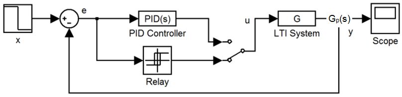
Figure 1: Relay feedback model
Describing function analysis
Fundamental to the understanding and application of the relay tuning techniques described as part of this paper is describing function analysis. This method of analysis was developed during the 1940s by Krylov and Bogolyubov (Krylov and Bogolyubov, 1947) during the search for an explanation as to why wartime gun- and antenna-tracking systems would oscillate about their set point. It was found that these oscillations arose from non-linearities in the systems such as those seen in gearing systems. An observation made was that when these oscillations occurred, the system output was often sinusoidal; hence the basis of the describing function technique is on the assumption of this case as presented by Atherton (Atherton, 2005).
A feedback system with a non-linearity is represented by the block diagram shown in Figure 2.
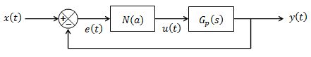
Figure 2: Block diagram representation of control system with a non-linearity
If the output u(t) of the above system is a sinusoidal limit cycle, then it may be assumed that the input to the non-linearity e(t) may also be sinusoidal. In this case, the fundamental of the output of the non-linear element N(a) can be calculated, with the higher harmonics neglected. It is these assumptions that are made in describing function analysis, with the non-linear element being defined as its gain to a sinusoidal input. In some cases the non-linear element may also phase shift the signal, hence the describing function may become complex.
The Fourier series is used to arrive at a describing function for a given non-linear element. In this case, the non-linear elements of particular interest are the relay and a relay with hysteresis. It is assumed that the input signal e(t) is a sinusoid:
The Fourier series representation of a periodic signal at the output y(t) is:
where:
As an assumption is made that the output of the non-linearity to be a sinusoid it is possible to say that the terms a0 and an are equal to zero because the output is symmetrical about the origin. Therefore the function is odd. Equation (3.2) now becomes:
Ideal relay
The ideal relay input/output relationship is shown in Figure 3, and represents an odd function, hence under Fourier analysis the coefficients A0 and An are zero.
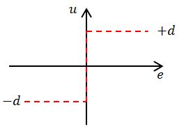
Figure 3: Input-output relationship for an ideal relay
For a relay of magnitude d, Equation (3.5) becomes:
For odd values of n this becomes, with combination of Equations (3.2) and (3.7):
Using the definition of the describing function as the ratio of the fundamental component (n=1) of the output of the non-linear element to the sinusoid input, we arrive at:
where N(a) is the describing function, an amplitude dependent gain-approximation non-linearity, as described above and a is an estimate of the amplitude of the fundamental component of the limit cycle.
It is important to note that the limit cycle frequency estimate, ω, given is more accurate than that for the amplitude, a (Atherton, 2011).
The ultimate gain can be determined by the intersection of the Nyquist curve and the negative inverse of the describing function. Hence, for an ideal relay, the ultimate gain is:
While the ideal relay provides an estimation of the critical frequency point, alternative relay types and configuration can be used to identify other points on the Nyquist curve.
Relay with hysteresis
A relay with hysteresis, ε has output d when its input reaches +ε, and output -d when its input reaches -ε as shown in Figure 4.
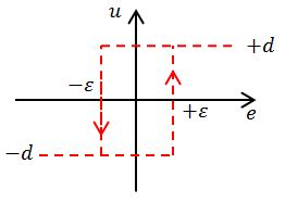
Figure 4: Input-output relationship for a relay with hysteresis
The describing function for a relay with hysteresis is given by:
and the identified point lies at the intersection of the Nyquist curve and a line parallel to the negative real axis. Through the variation of the hysteresis level, points at known phase shifts can be identified.
For this case it can be shown that the ultimate gain is equal to that for an ideal relay, as given by Equation (3.9).
Identification of additional points
Relay and transport delay
Artificial transport delay can be cascaded with a relay during a relay feedback test, as indicated by Figure 5.
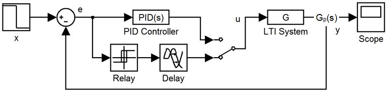
Figure 5: Relay-delay feedback model
This gives identification at a phase shift of:
where T is an arbitrary time delay. This method is the basis for an iterative time delay identification method (Chen et al., 2003).
Relay and integrator
When introduced into a feedback loop an integrator introduces a constant phase shift of -π/2 radians (Figure 6). It is this characteristic which can be used to identify the point on the frequency response at -π/2 radians. The slope of the magnitude curve is also modified.
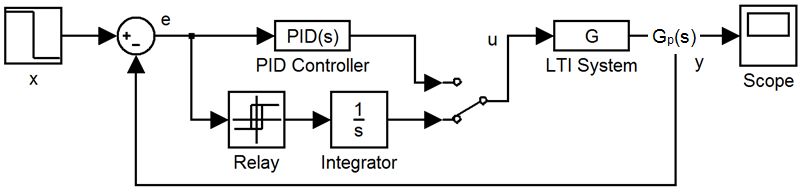
Figure 6: Relay-integrator feedback model
For a relay and integrator, the ultimate gain equivalent is given by:
where K-π/2 is the inverse of the process gain at the -π/2 radians point and ω-π/2 is the frequency at the same point.
Figure 7 gives a graphical representation of the previously described identification methods.
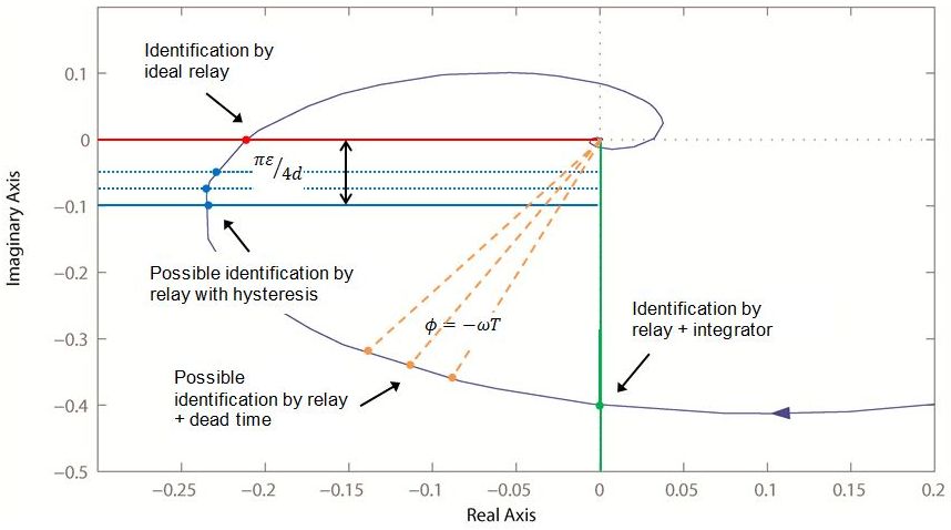
Figure 7: Graphical representation of multiple frequency response points identifiable with modified relay feedback
Improving Identification Accuracy
Due to the reliance on describing function analysis, errors in the recorded values of Ku result with a standard relay test. These errors are often in the region of 5 - 20% for typical transfer functions in a control system (Yu, 1999).
In this section, two methods are presented which aim to increase identification accuracy. Both methods aim to modify the relay output so that it becomes more sinusoidal.
While not discussed here, it is recognised that other methods for increased identification accuracy are in the literature. One of which is the use of a tuned filter (Atherton, 1999), for example, of the form with ωn close to the limit cycle frequency ω. This results in an almost sinusoidal limit cycle, hence reducing errors due to the assumptions made in describing function analysis.
Another useful method is in the application of bias to a relay in an iterative manner to counteract load disturbances as described by Yu (Yu, 1999) with use of Equation (4.1). This has been used later in practical experimentation.
where δo is the applied bias, h is the relay magnitude and Δa is the observed offset.
Relay with preload
Preload is applied as shown in Figure 8 (Tan et al., 2006). The principle behind this modification is to amplify the fundamental frequency relative to the other frequency components through the addition of the signal uk(t) to the input of the process.
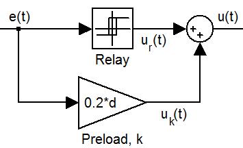
Figure 8: Addition of preload to a relay
If an input signal e(t)=asinωt is present, the addition of preload gives the amplitude of the first harmonic of the relay output as , where k is the preload gain. It is given that, with preload, the describing function becomes:
Hence the negative inverse of the describing function lies on the negative real axis as in the case of the ideal relay, but terminating at the point -1/k.
Ku is now calculated using Equation (4.3) and is equal to the describing function N(a) due to the fact that for the existence of a stable limit cycle there must be an intersection of Na and the process Nyquist curve. In addition, for this intersection to occur, is important to note that k must be smaller than Ku. ωu remains the frequency of the limit cycle.
Empirical studies (Tan et al., 2006) have shown that the preload gain should be 20-30% of the relay amplitude, hence where preload is used in this work it takes a value between:
Saturation relay
An alternative, more involved method is in the use of the saturation relay. Figure 9 shows the input-output relationship for a saturation relay.
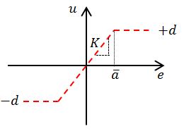
Figure 9: Input-output relationship for a saturation relay
This principle (Shen et al., 1996) again increases identification accuracy by amplifying the fundamental component at the relay output. This is achieved by the steady transition between the on and off states of the relay, which is defined by the value of the slope, K.
When the amplitude of the input reaches:
the relay output becomes ±d. That is:
Before this point the output is:
When
,
it can be shown that the describing function becomes:
To ensure that an intersection and hence limit cycle exists K must not become larger than . However, if the value of K is chosen to be too large, then the saturation relay becomes like the ideal relay and so its benefit is lost.
It is for this reason that it is recommended (Shen et al., 1996) that K should be set to:
,
where Ku is that recorded from an initial test with an ideal relay or K→∞. After the test is performed using the calculated value of K, the more accurate value of Ku is calculated using:
Methods for Controller Tuning
There are many hundreds of tuning methods available in the literature which make use of frequency points identified by relay feedback. Differences between these methods lie in the way that the identified frequency point in the Nyquist plot is manipulated or moved in order to create the desired closed loop response in the compensated system. Tuning methods have been selected from the simple and well-known to the more advanced and robust.
Single point tuning methods
PID phase margin method
The first tuning method considered is the original method presented by Åström and Hägglund (Åström and Hägglund, 1984a; Åström and Hägglund, 1984b) which utilises the identification of the ultimate gain and frequency, and allows a phase margin specification.
To gain suitable values for Td and Ti:
Td is given by:
where ϕm is the desired phase margin and kc is:
PI design method
In a similar manner, a PI controller can be designed through the identification of the frequency point at -π/2 radians, again giving a specification on phase margin.
Ti is given by:
and kc is:
where K-π/2 is the inverse of the process gain at the -π/2 radians point and ω-π/2 is the frequency at the same point.
It is important to recognise that because the frequency point at -π/2 radians is utilised this results in a compensated system with a lower closed loop bandwidth and a slower response when compared those methods which use the -π radians point, for a given system.
It is noted that the methods mentioned to this point have only one design criterion - the phase margin of the compensated system. While this gives a guaranteed frequency domain performance at the identified frequency it is not possible to predict the behaviour of the system around this frequency point. Hence, for more robust design more advanced methods are sought.
PID iso-damping method
A method designed with focus on a robust design is proposed (Chen et al., 2003). The basis of this method is in the specification on the slope of the Nyquist curve at the gain crossover frequency - in this case, the point at which the curve touches the sensitivity circle. The 'traditional' relationship between Ti and Td is modified from Ti=4Td to satisfy this condition which can be shown as:
,
where is the derivative of the slope of the Nyquist curve at the gain crossover frequency, ωc.
Historically, α in equation (5.1) has been set to 4, which originates from the popular Ziegler-Nichols tuning method (Nichols & Zeigler, 1942). The specific reason for this is not clear.
The design results in a Nyquist curve which is locally flat at the frequency ωc which gives a system which is more robust to changes in gain. This frequency is chosen by the designer and is recommended to be the desired cut-off frequency, hence allowing a greater degree of choice in the performance of the compensated system than a standard phase margin design. In this case, the desired frequency point is determined through a settling time specification (120 seconds), and related approximations (Appendix A). The frequency point is identified through an iterative gain method (Åström & Hägglund, 1984b).
The result will be a tuned system which will be relatively robust to changes in gain, and which will possess an 'iso-damping' property for changes in gain, that is, there will be very little change in overshoot under reasonable gain variations.
Td is given by:
where:
,
and sp(ω0) is defined as:
and, for the purposes of this method, are directly approximated using the Bode's integrals (Karimi et al., 2003) as:
where Kg is the steady-state gain of the process.
kc and Ti are given by:
Twin point enhanced Åström method
An alternative approach to achieving robust controller design is in the identification and use of more than one frequency point.
A twin-point tuning method (Tan et al., 1996) which aims to satisfy the shortcomings of the original Åström-Hägglund method is now presented. Again, as in the previous method, the traditional relationship between Ti and Td, where Ti=αTd, is modified. The first point used is the ultimate point (Ku, ωu), and the second is the point which corresponds to the phase margin ϕm which is to be designed for (kϕ, ωϕ). In addition, specification is put on the desired amplitude margin Am.
PID controller parameters are given by:
The attenuation factor r is recommended as:
where kϕ is the inverse of the magnitude at the point corresponding to the desired phase margin, while ωϕ is the frequency at this point.
This method gives a value of Ti so that the frequency response of the compensated system is attenuated at ω=ωu with attenuation dictated by r. That is:
Therefore, if r is increased, the resulting response will be more damped, whereas a smaller value for r will give a more oscillatory response. The recommended value of r is given above in Equation (5.14) where 0.9 represents 90% of its allowable range.
Coupled Tanks Apparatus
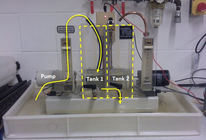
Figure 10: Coupled Tank Apparatus
The pictured (Figure 10) coupled tank apparatus was chosen to illustrate the various methods and techniques mentioned previously. The tank to the left is filled by a variable speed pump. On the adjoining wall between the two tanks there is an orifice which allows the fluid to flow between them. The level in each tank is measured by a hydrostatic pressure level device. At the front of each tank is a hand-operated valve which allows the fluid to exit and return to the reservoir. For the tests performed, only the valve on the right-most tank was opened (to a pre-defined point) during operation and the second pump was not used.
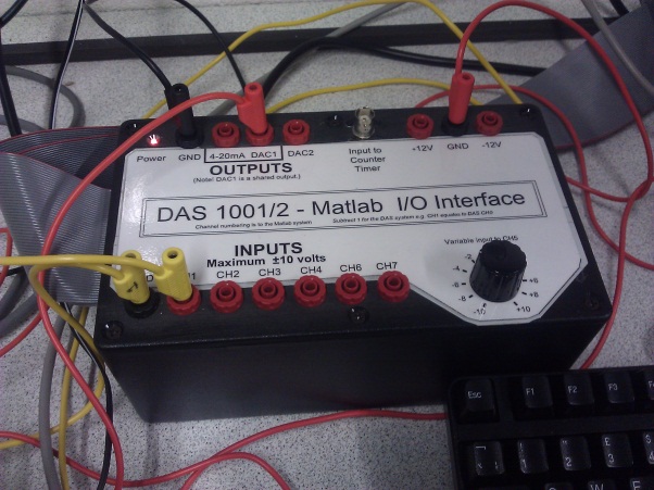
Figure 11: MATLAB I/O Interface
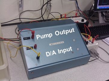
Figure 12: Voltage converter I/O unit
The input from the level device and the output to the pump was connected through an A/D and D/A breakout box (Figure 11) connected to a PC. In addition, the pump output passed through a further interface box (Figure 12) which supplied the correct voltage/current to the pump.
A Simulink model (Created by Dr Ian French, Teesside University) of the coupled tanks system was obtained, and is shown in Figure 13.
The Control System Toolbox® within Simulink was used to linearize the model in at an operating point corresponding to a voltage input from the level transducer of 4 volts, which was used throughout. The linearization function calculated the following transfer function for this operating point:
It can be seen that the transfer function is second order and has one dominant time constant, although one order of magnitude smaller than the time delay present.
As there was no approximation of dead time originally given with the Simulink model, a method by Wang and Shao (Wang and Shao, Autotuner based on gain- and phase-margin specifications, 1999; Wang & Shao, PID auto-tuner based on sensitivity specification, 2000) was adopted. This method gives an approximation of a system's dead time from frequency point identification at the -π and -π/2 points, coupled with use of the Newton-Raphson method.
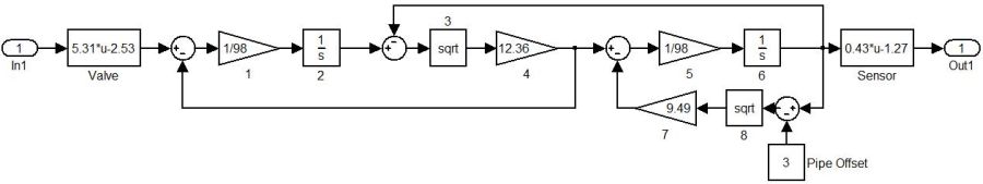
Figure 13: Simulink model of coupled tanks apparatus
The required relay feedback tests were performed, and with use of Equation (6.2), an initial estimate of θ=1.56 seconds was calculated. The Newton-Raphson iterative method was then applied with use of Equations (6.3) and (6.4), converging on a value of θ=1.84 seconds.
where:
It is noted that this value of dead-time is only strictly accurate for the operating point at which it was calculated (4V), although it is assumed that variation will be small enough to assume it applies over the whole operating range when needed.
Experiments performed
A number of relay feedback tests were performed with use of the coupled tanks rig. These are listed below:
- Ideal relay (Test 1)
- Ideal relay with preload (Test 2)
- Relay with hysteresis (Tests 3 & 4) (to counteract noise)
- Saturation relay (Tests 5, 8)
- Relay plus integrator (Tests 6-8)
From the above tests the following frequency points are identified:
- -π radians (Tests 1-5)
- -π/2 radians (Tests 6-8)
The result of Test 1 is shown graphically in Figure 14 with a selection of the remaining test results shown in Appendix B. It can be seen from Figure 16 that after approximately 75 seconds, the output y(t) settled into a steady limit cycle. The frequency and amplitude could then be measured over the subsequent 425 seconds to allow the calculation of the results shown in Table 1. In this case, a bias, δo, was applied to the relay as discussed in the next section.
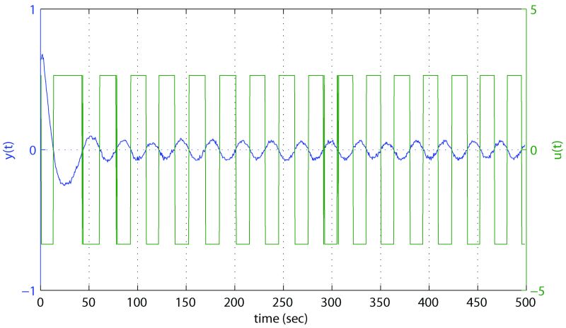
Figure 14: Relay feedback test results for Test 1
Notes on experimental methods
In some tests false switching of the relay was observed. This was particularly prevalent when the limit cycle amplitude was low and so the signal-to-noise-ratio (SNR) was low as in the case of Tests 1, 2 and 5. This unwanted effect was counteracted through first-order filtering, rather than hysteresis, as the former method was found to give superior results. An example of the benefit seen is given in Figure 15. Where load disturbances existed, a bias (δo) adjustment to the relay with use of Equation (4.1) was found increase accuracy greatly.
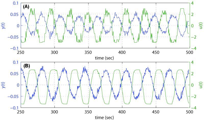
Figure 15: Comparison of relay feedback tests before (A) and after (B) additional filtering
To maximise accuracy, both amplitude (peak-to-peak) and frequency were measured manually, post-experiment, and averaged over at least three cycles, with data sampled through Matlab Real Time Workshop at an interval of 100ms. In cases where the limit cycle frequency was higher, measurements were averaged over more cycles, and sample interval increased accordingly.
In addition, as part of this work, a Simulink-based auto-tuner was developed that was able to automatically measure the required limit cycle parameters. This is discussed in detail in Appendix D.
Experimental Results
| Test | ε | d | k | 1s | Simulated | Linearized Model | Practical | |||||||||
|---|---|---|---|---|---|---|---|---|---|---|---|---|---|---|---|---|
| δo | ωc | a | Ku | |Gp(jω)| | ωc | |Gp(jω)| | δo | ωc | a | Ku | |Gp(jω)| | |||||
| 1. | - | 3.00 | - | No | -0.0786 | 0.1801 | 0.06852 | 55.75 | 0.0179 | 0.1930 | 0.0161 | -0.3600 | 0.2166 | 0.07080 | 53.95 | 0.0185 |
| 2. | - | 3.00 | 0.600 | No | -0.0786 | 0.1801 | 0.06889 | 56.04 | 0.0178 | 0.1930 | 0.0161 | -0.3600 | 0.2016 | 0.06836 | 56.48 | 0.0177 |
| 3.1 | 0.020 | 3.00 | - | No | -0.0749 | 0.1403 | 0.1111 | 34.38 | 0.0291 | 0.1470 | 0.0272 | - | 0.1878 | 0.09227 | 46.02 | 0.02429 |
| 4.1 | 0.020 | 3.00 | 0.600 | No | -0.0786 | 0.1403 | 0.1112 | 34.95 | 0.0286 | 0.1470 | 0.0272 | +0.014 | 0.1942 | 0.08301 | 46.62 | 0.02145 |
| 5.2,4 | - | 3.30 | - | No | -0.0690 | 0.1906 | 0.06387 | 60.65 | 0.0165 | 0.1930 | 0.0161 | +0.200 | 0.1963 | 0.06836 | 57.32 | 0.0175 |
| 6. | - | 0.005 | - | Yes | - | 0.01795 | 0.1627 | 0.0392 | 0.4579 | 0.0196 | 0.4600 | - | 0.0199 | 0.1636 | 0.0389 | 0.5114 |
| 7. | - | 0.005 | 0.001 | Yes | - | 0.01885 | 0.1670 | 0.0391 | 0.4818 | 0.0196 | 0.4600 | - | 0.0199 | 0.1684 | 0.0388 | 0.5128 |
| 8.3,4 | - | 0.005 | - | Yes | - | 0.01885 | 0.1466 | 0.0404 | 0.4663 | 0.0196 | 0.4600 | - | 0.0198 | 0.1928 | 0.0384 | 0.5032 |
Table 1: Summary of results at operating point Li = 4v
Notes:
Where preload is used, Ku is calculated using Equation (4.3)
1 Values quoted for modelled results take into account relay hysteresis, although the test is performed to estimate the ultimate point.
2 Saturation relay, K=1.4×55.87. Filtered t=1sec due to noise. Initial results with k=1×10⁶ as Test 2. Pump offset +6.3.
3 Saturation relay, K=1.4×1.94. Initial results with k=1×10⁶ as Test 3
4 Tabulated amplitude a and frequency ωc are those recorded after K is reduced
Discussion: identification accuracy
| Test No. | Test Description | Error (%) | Change in error (%) | ||
|---|---|---|---|---|---|
| Ku | ωu | Ku | ωu | ||
| 1 | Ideal Relay | -13.1 | 12.2 | 0.0 | 0.0 |
| 2 | Preload Relay | -9.1 | 4.5 | 4.1 | 7.8 |
| 3 | Ideal Relay with Hysteresis | -25.9 | -2.7 | -12.8 | 9.5 |
| 4 | Preload Relay with Hysteresis | -24.9 | 0.6 | -11.8 | 11.6 |
| 5 | Saturation Relay | -7.7 | 1.7 | 5.4 | 10.5 |
| 6 | Ideal Relay + Integrator | -10.1 | 1.5 | 0.00 | 0.00 |
| 7 | Preload Relay + Integrator | -10.3 | 1.5 | -0.25 | 0.00 |
| 8 | Saturation Relay + Integrator | -8.6 | 1.0 | 1.47 | 0.51 |
Table 2: Quantification of identification errors and increases in accuracy
N.B. Errors in Ku are calculated with use of Ku=|Gp(jω)|-1 from linearized model data.
Table 2 gives a quantification of error for each method versus calculated linearized model values. Changes in error give an indication of the benefits achieved by the application of hysteresis, preload and saturation relays. Changes are quoted with reference to Test 1 for Tests 2-5 and Test 6 for Tests 7 & 8. It is noted that in every case, the ultimate gain is underestimated, as expected due to describing function approximations.
It can be seen from Table 2 that the initial relay feedback test (Test 1) shows a good agreement with the expected modelled results. The addition of preload to the ideal relay (Test 2) gave a more accurate result for both Ku and ωu, with little effort required in terms of implementation complexity.
In Tests 3 and 4 it is seen that hysteresis had a significant effect on the results when compared to Test 1. The ultimate gain becomes smaller and more erroneous and the ultimate frequency estimation becomes more accurate when compared to Test 1, although it is thought that this result is incidental. When preload is used with hysteresis in Test 4 it can be seen that the frequency point estimation shows increased accuracy for Ku when compared to Test 3, while the estimation of ωu is very close to modelled values.
The use of the saturation relay in Test 5 provided the closest overall approximation to the modelled results. The time taken for this test is at least double that of the other tests due to the fact that an approximation of Ku has to be made before the saturation relay test can commence.
Tests 6-8 use an integrator to allow the identification of the -π/2 point on the frequency response. The duration of these tests was significantly longer (30 minutes) than those previous due to the much lower frequency of the limit cycle - a characteristic of the process. However, results, even with an ideal relay prove relatively accurate, with negligible improvement seen with the preload relay. With use of the saturation relay (Test 8), slightly better increase in accuracy is observed; however, this comes at a price of a test at a total duration of 60 minutes.
Identification accuracy and controller tuning
The results gained from the relay feedback tests in the previous section are now used for the tuning of PID-type controllers in order to ascertain the knock-on effects of identification inaccuracy on the ultimate performance of a controller.
Controllers are designed for each set of results using the original Åström-Hägglund PID phase margin design method to a phase margin specification of 60 degrees. The design results and measures of simulated performance in both frequency- and time-domains are given in Table 3.
It can be seen from Table 3 that the design exhibiting the best frequency response correlation to the model is that which made use of the saturation relay in the identification process. This is closely seconded by the method identifying the ultimate point with use of a preload relay. The remaining methods give close agreement in terms of phase margin, but don't agree so closely in terms of gain crossover frequency. This is mirrored in the responses shown in Figure 16, where these responses are seen to be slightly slower.
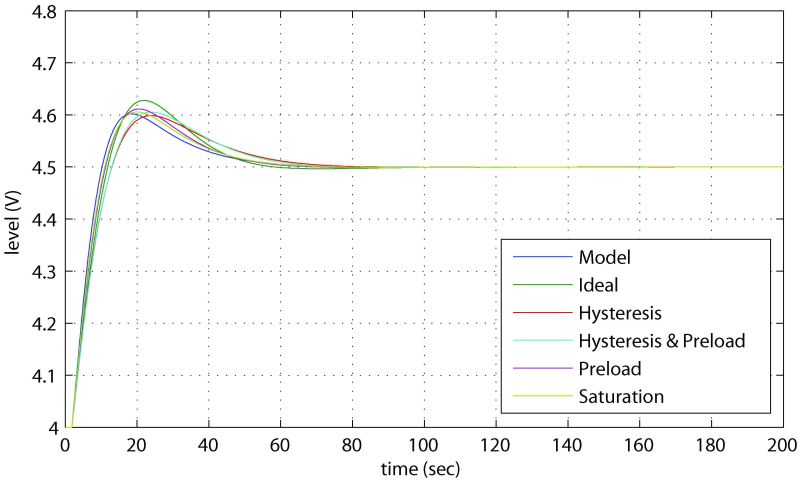
Figure 16: Simulated closed loop step response at operating point for PID controllers designed with 60° phase margin
| kc | Td | Ti | ϕm | ωg | ITAE | %OS | tS | |
|---|---|---|---|---|---|---|---|---|
| Linearized Model | 31.06 | 9.67 | 38.67 | 59.8 | 0.192 | 5.063 | 20.4 | 59.4 |
| Ideal Relay | 26.96 | 8.62 | 34.46 | 57.3 | 0.154 | 5.999 | 25.6 | 53.7 |
| Relay with hysteresis | 23.01 | 9.94 | 39.74 | 62.6 | 0.148 | 5.985 | 19.8 | 68.2 |
| Relay with hysteresis and preload | 23.31 | 9.61 | 38.43 | 61.4 | 0.146 | 6.071 | 21.0 | 65.5 |
| Relay with preload | 28.24 | 9.26 | 37.02 | 59.5 | 0.170 | 5.511 | 22.2 | 57.7 |
| Saturation Relay | 28.66 | 9.51 | 38.02 | 60.1 | 0.176 | 5.366 | 21.2 | 59.6 |
Table 3: PID parameters and performance evaluation for 60° phase margin
| Tuning Method | kc | Td | Ti |
|---|---|---|---|
| Ziegler-Nichols | 43.0 | 3.20 | 20.0 |
| Åström-Hägglund PID | 28.7 | 9.51 | 38.0 |
| PI Phase Margin | 1.72 | - | 87.9 |
| Iso-damping1 | 2.00 | 9.00 | 46.1 |
| Enhanced Åström2 | 4.22 | 3.17 | 159 |
Table 4: Calculated controller parameters for proposed tuning methods
1 the steady state gain, kg=1.43, is estimated using a biased relay (Shen et al., 1996)
2 the attenuation factor used is equal to 85% of the allowable limit, r=11.70
Tuning methods
In order to compare the previously proposed tuning methods, controllers are designed for each, as well as a simple tuning with use of the Ziegler-Nichols rule to act as a reference. Where appropriate, identifications performed with the saturation relay in the previous section are used, due to earlier findings. Appendix A gives details of the design decisions and criterion applied in each case.
The controller parameters are given in Table 4. Each controller has been implemented on the coupled tanks rig, except for the Åström PID design. This was not realisable due to a large derivative action, which resulted in excessive noise at the controller output. For this controller, simulated results are given where appropriate. In the remaining cases a PID controller with output limiting via clamping was used to prevent integral windup. Appendix C gives simulated and practical closed loop step responses for each case.
To improve data collected from the coupled tanks rig, which had reasonable noise content, smoothing using a 3rd order Savitzky-Golay least-squares smoothing filter was performed in Matlab. This filter works by fitting a polynomial to a frame of noisy data. The frame length chosen in this case is 101 data points, which equates to 5 seconds of data at the sampling time of 0.05 seconds.
Discussion: tuning results
The frequency domain performance measures in Table 5 indicate that the designs have been largely successful. For the Ziegler-Nichols controller the step response is overly oscillatory. This is expected considering the low phase margin which has resulted. Additionally, upon implementation, a large amount of actuator saturation is experienced, resulting in an unpredictable step response which is not desirable.
The Åström PI controller gives the slowest response with the longest settling time and relatively large ITAE result, although overshoot is relatively small. This slow response is due to the nature of the design method which allows no specification other than phase margin and a low value for ωg which is found on the negative real imaginary axis. While the response is poor in terms of speed, it must be noted that such a conservative design ensures that no actuator saturation occurs, which may be beneficial in some circumstances.
The next longest settling time is seen from the iso-damping method which also exhibits the largest overshoot and ITAE measure. In design, a settling time of 120 seconds was specified with an overshoot of approximately 10%, hence, the design has not met these specifications. It is thought that this is due to the nature of the approximations used which assumed dominant complex poles. However, the phase margin specification is been met within reasonable limits.
| Tuning Method | kc | Td | Ti | Performance Measures | ||||
|---|---|---|---|---|---|---|---|---|
| ϕm | Am | %OS | ts | ITAE | ||||
| Ziegler-Nichols* | 43.0 | 3.20 | 20.0 | 18.4 | 7.16 | 11.0 (66.6) | 141 (147) | 12.9 (41.9) |
| Åström PID*† | 28.7 | 9.51 | 38.0 | 60.1 | 4.84 | 24.3 (15.6) | 129 (68.9) | 12.6 (5.23) |
| Åström PI | 1.72 | - | 87.9 | 60.5 | 29.9 | 10.4 | 428 | 32.6 |
| Iso-Damping | 2.00 | 9.00 | 46.1 | 47.6 | 72.4 | 24.6 | 397 | 33.6 |
| Enhanced Åström | 4.22 | 3.17 | 159 | 63.8 | 72.4 | 3.20 | 191 | 15.1 |
Table 5: Comparison of practical results for tuned controllers
*pump saturation experienced on coupled tanks rig, values in parentheses are under simulation without saturation
† values quoted for Åström PID are under simulation as controller is unrealisable
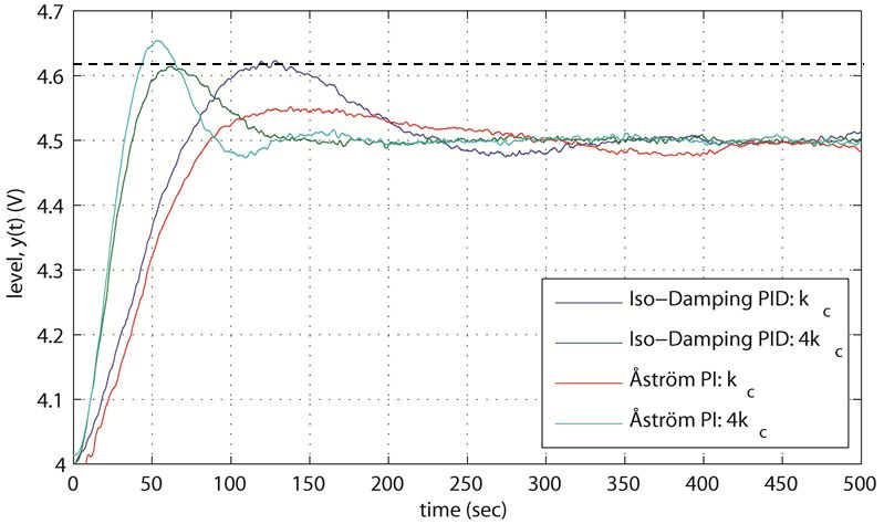
Figure 17: Step tests demonstrating the achieved iso-damping property
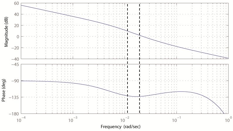
Figure 18: Bode diagram for iso-damping compensated coupled tanks system
However, a merit of this method lies in the possibility of improving quality of the time-domain performance through specification of the frequency ωc, should this be required. Although the time domain performance lacks somewhat, the iso-damping quality for which the controller was primarily designed is apparent. Figure 17 shows that, due to the flat phase condition designed for, a large change in loop gain has very little effect (approx. +1.0%) on the amount of overshoot seen, in comparison with the Åström PI controller which exhibits an increase of +20.4%. The cause of this small change in overshoot, the flat phase condition, can be seen in Figure 18.
The best time-domain performance is given by the Enhanced Åström design. In addition, this method ensures a robust design through the shaping of the frequency response. However, it is noted that the amplitude margin specification was not met, possibly due to the presence of dead-time in the plant.
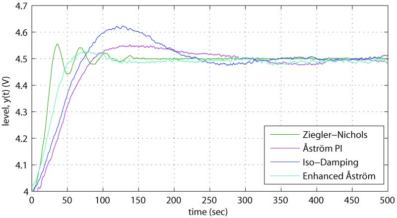
Figure 19: Comparison of step responses for the coupled tanks apparatus with controllers tuned using various frequency response methods
Conclusion
In this paper, two main considerations have been made. The first relates to methods for increasing frequency point identification, while the second relates to the subsequent use of these identified points for controller tuning. The most important findings are summarised here.
The use of both preload and saturation relays gave increases in estimation accuracy for Ku and ωu in application on the coupled tanks rig at the ultimate point, with superior results seen for the saturation relay. Much smaller increases were seen at the -π/2 point for both methods. Due to the findings made, the preload relay is recommended for the identification of all points due to very little additional effort required for its implementation.
In most industrial applications, the desire is often for a method which minimises both process disturbance and the potential for lost production, and hence, profit. Due to this and as the practical implementation of the saturation relay is relatively time-intensive, it is concluded that its implementation should not be necessary in the majority of cases, as the benefit it gives over the preload relay may often not be sufficient.
In the case of the coupled tanks rig used it was found that the best way to counteract noise while maintaining accuracy was through filtering, rather than hysteresis. Where load disturbances existed, a simple bias adjustment to the relay was found increase accuracy greatly.
A variety of tuning methods have been discussed. The main limitation of the simple methods first given by Åström and Hägglund is shown in the fact that the frequency at which tuning occurs is fixed. This has given rise to problems relating to excessive derivative action, actuator saturation and sluggish responses. Through implementation of more advanced methods, superior performance in the time- and frequency-domains has been seen, in particular in the case of the Enhanced Åström method.
Finally, techniques such as the iso-damping method have illustrated the robust design capabilities of relay auto-tuning technique where negligible overshoot increases were seen for relatively large changes in loop gain.
In the light of these findings, it is concluded that, for the vast majority of cases, where average performance is required, a simple, fast tuning using the original methods proposed by Åström and Hägglund may suffice. However, where applications demand, methods which give superior responses are available, although much more application effort is required. With the coupled tanks rig or similar in mind, and while considering the findings made in this paper, the preload relay method for identification coupled with the iso-damping method for controller tuning would be recommended.
Recommendations For Further Work
The potential for further work in this area is vast. Studies could be conducted relating to more recent identification methods like that by Je et al. which uses optimally combined pulses for frequency point identification (Je et al., 2009). Although not mentioned in this paper, based on Wang and Shao (Wang and Shao, 1999; Wang and Shao, 2000), investigations could be performed into advanced system identification methods (Wang et al., 1999) which adopt FFT methods to for simultaneous multiple point identification. Finally, work could be carried out with focus on the possibility of increasing the accuracy of the relay with hysteresis with incorporation of the preload relay.
Acknowledgements
With thanks to Michael Short for his supervision, time, and advice; Ian French for guidance and the provision of the coupled tanks rig model; John Mudd for assistance relating to laboratory equipment.
List of Figures
Figure 1: Relay feedback model
Figure 2: Block diagram representation of control system with a non-linearity
Figure 3: Input-output relationship for an ideal relay
Figure 4: Input-output relationship for a relay with hysteresis
Figure 5: Relay-delay feedback model
Figure 6: Relay-integrator feedback model
Figure 7: Graphical representation of multiple frequency response points identifiable with modified relay feedback
Figure 8: Addition of preload to a relay
Figure 9: Input-output relationship for a saturation relay
Figure 10: Coupled Tank Apparatus
Figure 11: Matlab I/O Interface
Figure 12: Voltage converter I/O unit
Figure 13: Simulink model of coupled tanks apparatus
Figure 14: Relay feedback test results for Test 1
Figure 15: Comparison of relay feedback tests before (A) and after (B) additional filtering
Figure 16: Simulated closed loop step response at operating point for PID controllers designed with 60° phase margin
Figure 17: Step tests demonstrating the achieved iso-damping property
Figure 18: Bode diagram for iso-damping compensated coupled tanks system
Figure 19: Comparison of step responses for the coupled tanks apparatus with controllers tuned using various frequency response methods
List of Tables
Table 1: Summary of results at operating point Li = 4v
Table 2: Quantification of identification errors and increases in accuracy
Table 3: PID parameters and performance evaluation for 60° phase margin
Table 4: Calculated controller parameters for proposed tuning methods
Table 5: Comparison of practical results for tuned controllers
Appendix A: Notes on Controller Design
Åström and Hägglund PI/PID methods
In the case of the Åström-Hägglund PID and PI methods, a phase margin of 60 degrees was chosen, as this is within recommended limits.
Iso-damping method
For the iso-damping method, and based on the closed loop performance achieved using the Ziegler-Nichols rule, the design was performed for a settling time of 120 seconds and an overshoot of 10%. This was achieved through the assumption of second-order dominant poles and related equations as shown below:
To find settling time, or find the natural frequency to give a particular settling time with known ζ:
Then, as found in (Richter, 2009):
To find bandwidth frequency, ωb, for 0.3≤ζ≤0.8:
Then, the crossover frequency can be found using a rule of thumb:
Another rule of thumb (Choudhury, 2005) used is:
In this case, designing for a settling time of 120 seconds and , hence
overshoot. Therefore,
,
, which gives
.
In order to identify the frequency point at the required frequency, an iterative gain method proposed by Åström and Hägglund (Åström and Hägglund, 1984b) was used.
Additionally, this method required an estimate of steady state gain Kg for the plant. For this, a method presented in (Shen et al., 1996) where a bias is applied to a relay and the steady-state gain is given by:
Enhanced Åström method
In this case a phase margin of 60 degrees and an amplitude margin of 1 were selected. The -2π/3 radians point was identified, again, with the Åström iterative gain method (Åström and Hägglund, 1984b). The attenuation factor r, was decreased to 85% of its allowable range (Tan et al., 1996) in order to optimise time-domain performance.
Appendix B: Relay Feedback Tests
The following figures show examples of the relay feedback tests performed on the coupled tanks rig:
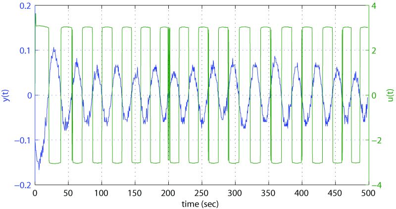
Figure B-1: Relay feedback test results for Test 2
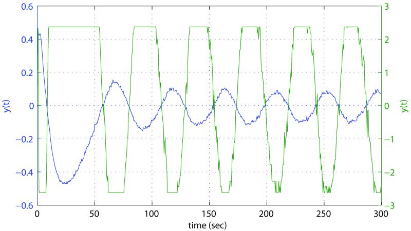
Figure B-2: Relay feedback test results for Test 5
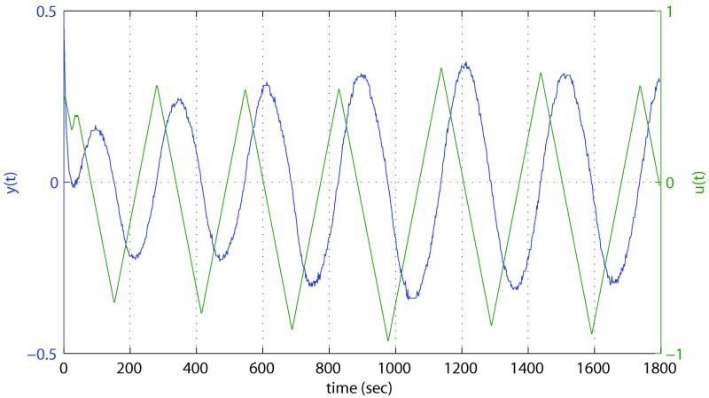
Figure B-3: Relay feedback test results for Test 6
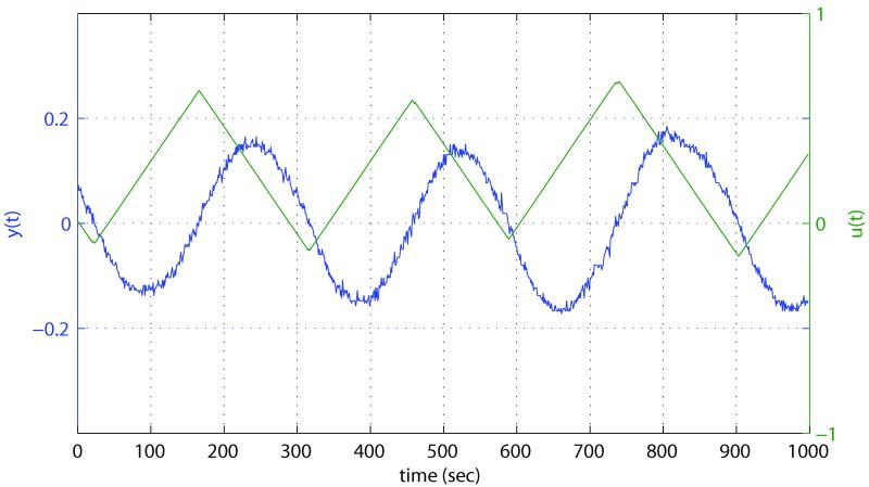
Figure B-4: Relay feedback test results for Test 7
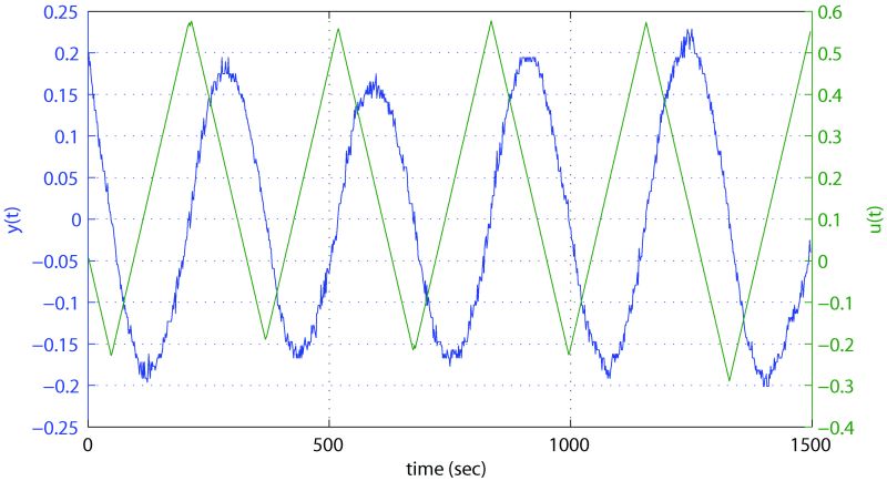
Figure B-5: Relay feedback test results for Test 8
Appendix C: Tuning Results
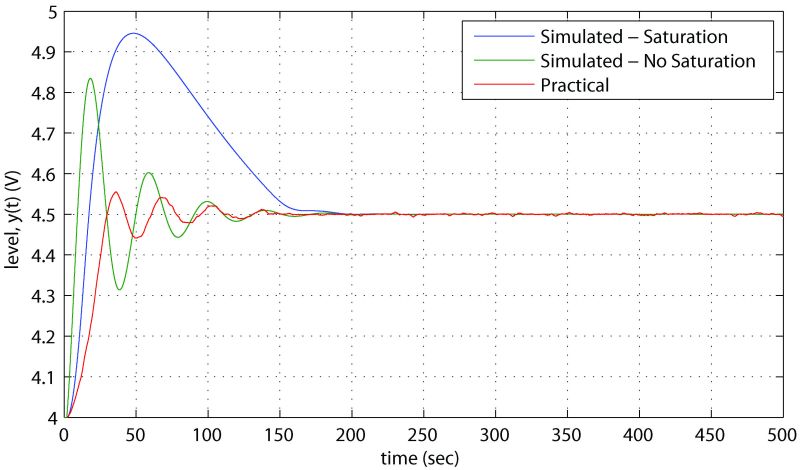
Figure C-1: Comparison between practical and simulated response to a change in set point for the designed Ziegler-Nichols controller
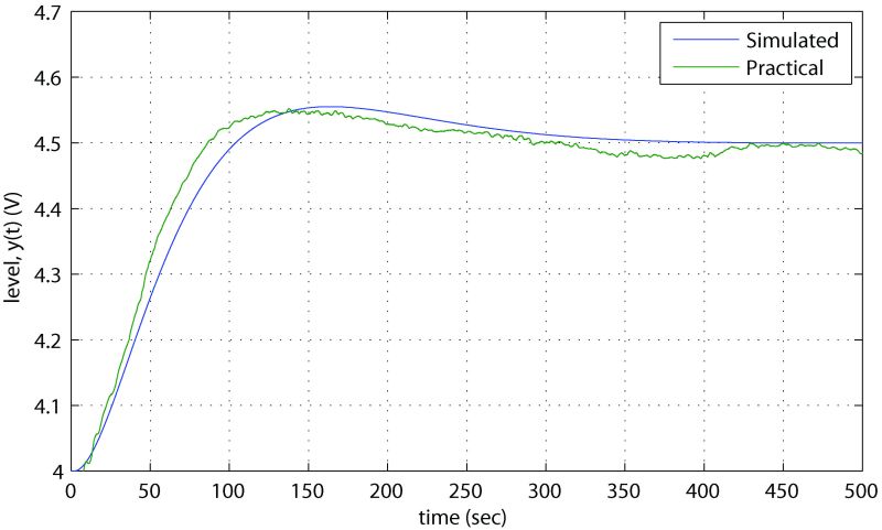
Figure C-2: Comparison between practical and simulated response to a change in set point for the designed Åström PI controller
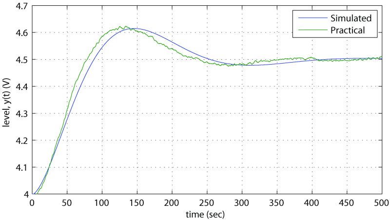
Figure C-3: Comparison between practical and simulated response to a change in set point for the designed iso-damping PID controller
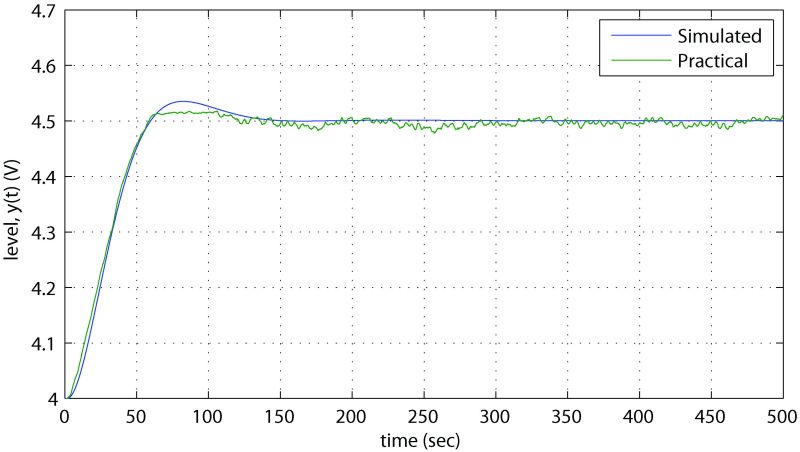
Figure C-4: Comparison between practical and simulated response to a change in set point for the designed Enhanced Åström PID controller
Appendix D: Simulink-Based One-Button PID Auto-Tuner
To aid in the analysis and simulation during this work, various Simulink-based auto-tuning models were developed relating to many of the methods studied. Initially, a basic model was designed to measure the amplitude and frequency of the limit cycle, and subsequent developments provided the ability to calculate PID parameters.
Inspiration for the measurement of frequency and amplitude was taken from Åström and Hägglund (Åström and Hägglund, 1984a) who suggest this may be possible simply by measuring zero crossings and maximum and minimum signal values.
Through much development and testing, we arrive at the model faceplate shown in Figure D-1. This model incorporates a PID controller and relay auto-tuner based on the Åström PID design, and allows specification of hysteresis should this be desired. The user is able to select the times at which the tuning begins and stops. Upon completion of the tuning, the model updates the parameters of the PID controller with the ones just calculated.
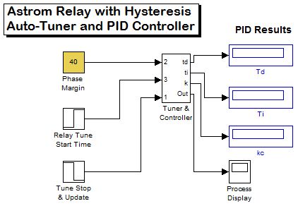
Figure D-1: Faceplate of auto-tuner Simulink model
Figure D-2 gives a view inside the 'Tuner and Controller' subsystem shown in Figure D-1. Here the PID, controller, simulated plant, and Åström auto-tuner subsystem can be seen. A switch can also be seen which provides a transition between the relay test and control activation. Bumpless transfer has been included in the PID block to ensure that the plant does not undergo a large disturbance during the transition between the relay test and the activation of control with the updated PID parameters provided by the 'PID Update Switch' block, which is triggered by the test stop signal in Figure D-1.
Figure D-3 shows the internals of the crucial 'Åström Autotuner' subsystem which is used to perform the calculations of Ku, ωu and subsequently the PID parameters. This subsystem was the original model with which measurements were performed for examples given earlier in this report. The limit cycle signal is input through Input 1. Input 3 controls the start time of the measurements, and is connected to the start input in Figure D-1. Input 4 is taken from the set point of the process and applied a bias to the measured signal, ensuring it is centred on zero.
Frequency is measured through use of a zero crossing block, which counts the number of zero crossings which occur during a given time period. Time is measured through a counter connected to a signal generator set at 1Hz. Simulation time is not useful in this case due to the choice of start time through Input 3. The number of zero crossings is then divided by the time over which the count was taken. Subsequently calculations are applied to arrive at ωc and fc.
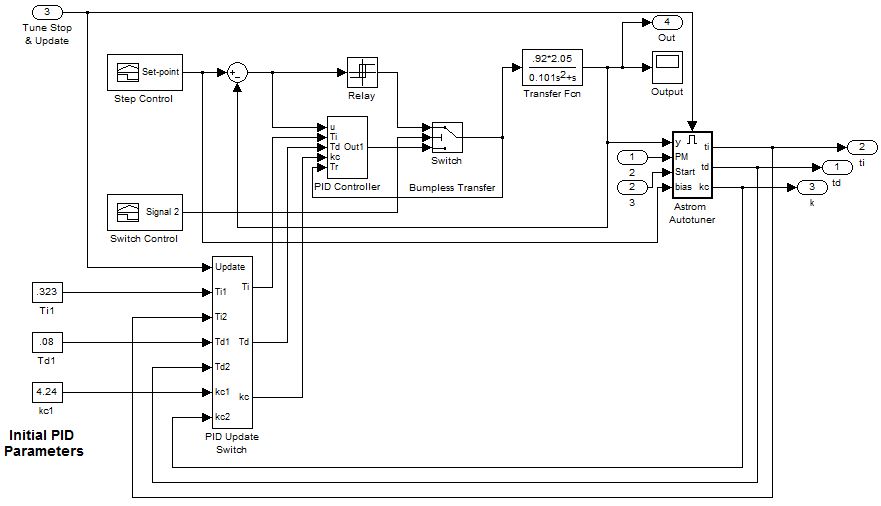
Figure D-2: 'Tuner and Controller' subsystem within auto-tuner
Amplitude is measured through the simple measurement of the maximum and minimum values of the signal, which are averaged to give a and manipulated to give Ku providing the correct value of d is present in block 'Fcn2'. This measurement also starts when Input 3 becomes true.
The last portion of the model is concerned with the calculation of the PID parameters to a phase margin specification, and uses an embedded Matlab function to apply the Åström calculations to the values measured previously. Options for varying the ratio Ti/Td and specifying the amount of relay hysteresis present are provided which alter the calculations accordingly. Phase margin is set outside the auto-tuner subsystem, as seen in Figure D-1.
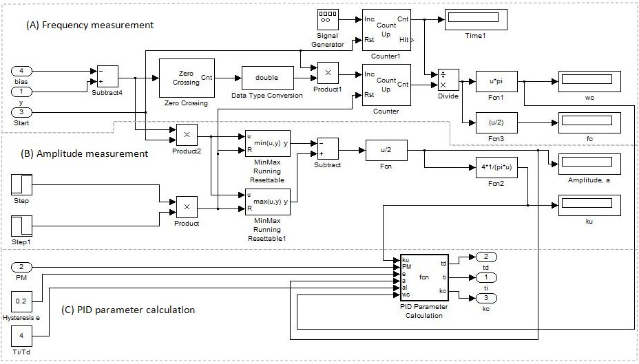
Figure D-3: Main subsystem within Åström-Hägglund auto tuner model
The model is demonstrated, in simulation, for the coupled tanks rig. The PID controller is initially tuned with the parameters given by the Ziegler-Nichols method and a step is applied at 10 seconds. A relay feedback test is performed from 250 - 700 seconds, with measurements starting at 450 seconds. A specification of 60° phase margin is set, PID parameters are calculated and the controller is updated at 700 seconds. At 800 seconds, another step is applied, where the change in controller performance is seen. The new PID parameters are [kc, Td, Ti]=[28.2, 10.6, 42.4], very similar to the results given in Table 3. The plant output over this time range is shown in Figure D-4.
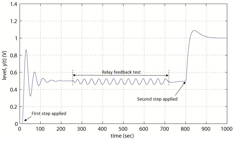
Figure D-4: Output of relay auto-tuner model
Notes
[1] Stephen Hornsey recently graduated from Teesside University with BEng Instrumentation and Control Engineering. He now works as an Instrument Electrical Engineer for SABIC UK Petrochemicals Ltd. on a world-scale high-pressure tubular low-density polyethylene plant in the North East of England.
References
Argelaguet, R. (1996), 'A new tuning of PID controllers based on LQR optimisation', in Preprints of Proceedings of PID '00: IFAC Workshop on Digital Control, pp. 303–308
Åström, K. J. and T. Hägglund (1984a), 'Automatic tuning of simple regulators', in Proceedings of IFAC 9th World Congress, Budapest, pp. 1867-72
Åström, K. J. and T. Hägglund (1984b), 'Automatic tuning of simple regulators with specification on phase and amplitude margins', Automatica, 20, 645-51
Åström, K. J. and T. Hägglund (1984c), 'A frequency domain method for automatic tuning of simple feedback loops', in Proceedings of the 23rd IEEE conference on decision and control, Las Vegas, pp.299-304
Åström, K. J. and T. Hägglund (1988), Automatic tuning of PID controllers, NC: Instrument Society of America
Åström, K. J. and T. Hägglund (1995), PID Controllers: Theory, design, and tuning, Research Triangle Park, N.C.: International Society for Measurement and Control
Atherton, D. P. (2005), Control of Nonlinear Systems, available at http://www.atp.ruhr-uni-bochum.de/rt1/nonlin/, accessed 12 March 2011
Bialkowski, W. L. (1993), 'Dreams versus reality: A view from both sides of the gap', Pulp and Paper Canada, 94, 19-27
Bristol, E. H. (1977), 'Pattern recognition: an alternative to parameter identification in adaptive control' Automatica, 13, 179-202
Chen, Y., C. Hu and K. Moore (2003), 'Relay feedback tuning of robust PID controllers with iso-damping property', in 42nd IEEE conference on decision and control, Maui: IEEE
Choudhury, D. (2005), Modern Control Engineering, New Delhi: Prentice-Hall
Cohen, G. H. and G. A. Coon (1953), 'Theoretical consideration of retarded control', Transactions of the American Society of Mechanical Engineers, 76, 827-34
Dormido, S. and F. Morilla (2000), 'Methodologies for the tuning of PID controllers in the frequency domain', Proceedings of IFAC workshop on digital control, pp. 155-160
Dormido, S. and F. Morilla (2004), 'Tuning of PID controllers based on sensitivity margin specification', in Proceedings of 5th Asian Control Conference, Melbourne, Australia, 1, 486-491
Ender, D. B. (1993), 'Process control performance: Not as good as you think', Control Engineering, 9, 180-90
Friman, M. and K. V. Waller (1997), 'A two-channel relay for autotuning', Industrial Engineering Chemistry Research, 36, 2662-71
Garcia, C. E. and M. Morari (1982), 'Internal Model Control: A unifying review and some new results', Industrial & Engineering Chemistry Process Design and Development, 1, 308-23
Hang, C. C., K. J. Åström and W. K. Ho (1991), 'Refinements of the Ziegler-Nichols tuning formula,' Control Theory and Applications, IEE Proceedings D, 21, 111-18
Hang, C. C., K. J. Åström and W. K. Ho (1993), 'Relay auto-tuning in the presence of static load disturbance', Automatica, 29, 563-64
Hang, C. C., H. T. Lee and W. K. Ho (1993), Adaptive Control, North Carolina: Instrument Society of America
Ho, W. K., O. P. Gan, E. B. Tay and E. L. Ang (1996), 'Performance and gain and phase margins of well-known PID tuning formulas,' IEEE Transactions on control systems technology, 4, 473-77
Je, C. H., J. Lee S. W. Sung and D. H. Lee (2009), 'Enhanced process activation method to remove harmonics and input nonlinearity', Journal of Process Control, 19(2), 53-57
Jeon, C. H. et al., (2010), 'Relay feedback methods combining sub-relays to reduce harmonics', Journal of Process Control, 20(1), 228-34
Krylov, N. and N. Bogolyubov (1947), Introduction to Nonlinear Mechanics, Princeton: Princeton University Press
Lin, J. Y. and C. C. Yu (1993), 'Automatic tuning and gain scheduling for pH control', Chemical Engineering Science, 48, 3159-71
Liu, G. P. and S. Daley (2001), 'Optimal-tuning PID controller design in the frequency domain with application to a rotary hydraulic syste', Control Engineering Practice, 7, 1185-94
Murray, R. M. and K. J. Astrom (2008), Feedback Systems: An Introduction for Scientists and Engineers, Princeton: Princeton University Press
Nichols, N. B. and J. G. Zeigler (1942), 'Optimum settings for automatic controllers', Transactions of the ASME, 64, 759-68
Papastathopoulou, H. S. and W. L. Luyben (1990), 'Potential pitfalls in ratio control schemes', Industrial Engineering & Chemical Research, 29, 2044-53
Pessen, D. W. (1994), 'A new look at PID-controller tuning', Transactions of the American Society of Mechanical Engineers, Journal of Dynamic Systems, Measurement and Control, 116, 553-57
Radke, F. and R. Isermann (1987), 'A parameter-adaptive PID controller with stepwise parameter optimisation', Automatica, 23, 449-57
Richter, H. (2009), Relative stability: gain and phase margins & frequency domain performance, Cleveland: Cleveland State University
Seborg, D. E., T. F. Edgar and D. A. Mellichamp (1989), Process Dynamics and Control, New York: Wiley
Shen, S. H., J. S. Wu and C. C. Yu (1996), 'Use of biased-relay feedback for system identification', AIChE Journal, April, 42(4), 1174-80
Shen, S., H. Yu and C. Yu (1996), 'Use of saturation-relay feedback for autotune identification', Chemical Engineering Science, 51, 1187-98
Sung, S. W. and J. Lee (2006), 'Relay feedback method under large static disturbances', Automatica, 42, 353-56
Tan, K. K. et al., (2006), 'Improved critical point estimation using a preload relay', Journal of Process Control, 16(5), 445-55
Tan, K. K., T. H. Lee and Q. G. Wang (1996), 'Enhanced automatic tuning procedure for process control of PI/PID controllers', AIChE Journal, 42(9), 2555-62
Wang, Q. G., C. C. Hang and Q. Bi (1997), 'A frequency domain controller design method', Transactions of the Institution of Chemical Engineers, 64-72
Wang, Q. G., C. C. Hang and Q. Bi (1999), 'FFT-based frequency response identification from relay feedback', Automatica
Wang, Q. G., T. H. Lee and C. Lin (2003), Relay Feedback: Analysis, Identification and Control, Gateshead: Springer-Verlag
Wang, Y. and H. Shao (1999), 'Autotuner based on gain- and phase-margin specifications', Industrial & Engineering Chemistry Research, 45, 3007-12
Wang, Y. and H. Shao (2000), 'PID auto-tuner based on sensitivity specification', Transactions of the Institute of Chemical Engineers, 78(A), 312-16
Wood, R. K. and M. W. Berry (1973), 'Terminal composition control of a binary distillation column', Chemical Engineering Science, 28, 1707-17
Yu, C. C. (1999), Autotuning of PID Controllers, New York: Springer-Verlag
To cite this paper please use the following details: Hornsey, S. (2012), 'A Review of Relay Auto-tuning Methods for the Tuning of PID-type Controllers', Reinvention: an International Journal of Undergraduate Research, Volume 5, Issue 2, www.warwick.ac.uk/reinventionjournal/issues/volume5issue2/hornsey Date accessed [insert date]. If you cite this article or use it in any teaching or other related activities please let us know by e-mailing us at Reinventionjournal at warwick dot ac dot uk.