Border Effects Among EU Countries: Do National Identity and Cultural Differences Matter?

Mantas Vanagas ^[1], Department of Economics, University of Warwick

Abstract

This article analyses how national borders affect trade patterns among the European Union countries. We estimate that domestic trade of European countries is 7.5 times bigger than international trade. The border effects for the countries which joined the EU in 2004 exhibit a sharp decline, suggesting that European policies and institutions effectively help countries to integrate into the single market. Other authors find that nationalism and cultural differences are positively related to consumer preferences for domestically produced goods. We raise a hypothesis that these factors might explain the border effect puzzle. The results show that both nationalism and cultural differences have an impact on border effects.

Keywords: International trade, border effects, EU countries, nationalism, cultural differences.

Introduction

Globalisation, various free-trade agreements and European integration suggest that national borders should have very little or no impact on trade patterns. However, economists observe border effects, which are defined as 'the extent to which the volume of domestic trade exceeds the volume of international trade' (Evans, 2003: 1291). McCallum (1995) estimated a surprisingly high border effect for trade flows between US and Canada. His findings sparked a debate regarding its potential causes and implications. Obstfeld and Rogoff (2000) named the border effect as one of the 'six major puzzles in international economics'.

Different authors in the trade literature have tried to explain why estimated border effects are unexpectedly high. A high degree of substitution between domestic and foreign goods (Evans, 2003), trade barriers (Wei, 1996; Hillberry, 1999; Head and Mayer, 2000; Wolf, 2000; Chen, 2004) and problems in the standard methodology (Anderson and van Wincoop, 2003; Head and Mayers, 2002) are the most widely researched reasons. This article takes a different approach and analyses border effects in the context of consumer preferences. The fact that consumers simply gain more pleasure from consuming domestically produced goods can be a missing part in the border effect explanation.

This article has two major objectives. First, it provides estimates of border effects among European Union countries. One of the cornerstones of the European Union is the idea of a single market; there have been no tariffs and quotas within the EU since 1968. In addition the European Commission has adopted a number of policies, such as the Single Market Programme, in order to eliminate non-tariff trading barriers and to encourage market integration (Head and Mayer, 2000: 284-85). This article assesses the extent and dynamics of market fragmentation in the EU by estimating the border effects and what has happened to them over time. More rigorous knowledge about the reasons for border effects in the European Union might contribute to a more successful implementation of integration policies. If border effects arise due to an optimal behaviour of companies and individuals then no additional policy intervention is needed. However, if border effects are a result of some trade frictions and barriers, welfare improvement can be achieved (Chen, 2004: 94).

Secondly, we establish a relationship between border effects and nationalism as well as cultural differences among countries. A series of authors in marketing literature define a consumer behaviour property called consumer ethnocentrism, which manifests as a tendency to favour domestic goods because of a belief that buying foreign goods harms the domestic economy (Shimp and Sharma, 1987: 280). Belabanis et al. (2001) investigate the relationship between national identity variables (nationalism, patriotism and multi-nationalism) and consumer ethnocentricity. If border effects reflect consumer preferences then we would expect that nationalism and cultural differences might also contribute to the explanation of border effects.

In this article we will explain data and methodology; provide a thorough analysis of border effects and their dynamics; investigate border effects sensitivity to domestic distances; analyse the relationship between nationalism and border effects; examine cultural differences and discuss potential endogeneity problems, before concluding.

Data and methodology

A panel dataset was collected from two main data sources to estimate the implied border effects (for more details about data and variables see Appendix 1). Bilateral trade data and total gross output, needed to estimate domestic trade, were obtained from the OECD statistics database. All the other variables were acquired from the World Bank's World Development Indicators database. The dataset includes observations for 18 members of the European Union plus Norway and Switzerland at three points in time: 1995, 2000 and 2005. Although Switzerland and Norway do not belong to the EU, they have adopted many EU policies and are closely linked in terms of trade with other EU countries. For this reason we refer to all the sample countries as EU members. Bilateral trade data availability does not allow us to expand the number of countries to the full list of EU members. The choice of the countries implies that no border-related tariffs exist among these countries.

This article uses a standard gravity model:

$\ln(trade_{ij}) = \alpha_0 + \alpha_1\ln(GDP_i) + \alpha_2\ln(GDP_j) + \alpha_3\ln(distance_{ij}) + \alpha_4\ln(Remoteness_{ij})$

$\qquad + \alpha_5\ln(Remoteness_{ji}) + \alpha_6home_i + \varepsilon_{ij}$

The dependent variable is a bilateral trade flow. It measures the value of goods exported from country i to country j. It is important to note, for some observations of the bilateral trade flow, variable measure domestic trade. This follows Wei's (1996: 3) proposal, where domestic trade flows are treated as country's export to itself. Consequently, there are two types of trade: international trade, a control group within which every trade flow crosses a country border at least once, and domestic trade, i.e. a treatment group. Countries are expected to trade more with each other the larger they are. This is measured by gross domestic product of exporter and importer. The distance variable indicates that more distant countries tend to trade less as transportation costs rise. The economic remoteness variables, as Helliwell (1997: 169-70) explains, play an important role as well. They are defined as

$remoteness_{ij} = \Bigg(\sum_{j,j\neq{i}}\frac{GDP_j}{distance_{ij}}\Bigg)^{-1}$

The volume of trade between two countries depends not only on their size and the distance from each other, but also on the size and the distance to other trading partners. For example, the fact that France, a strong economy, is close to Spain might have an impact on a trade volume between Spain and Portugal, because some goods produced in Spain, which might otherwise have been directed to Portugal, are exported to France. Home variable is a dummy that takes value 1 for domestic trade and 0 for international trade flows. A measure of interest, the border effect, is

$border e\!f\!f\!ect = exp(\alpha_6)$

It captures the difference in the magnitude of the average domestic trade volume relative to international trade flow.

Empirical results

Table 1 presents the results of the estimated gravity equation. Equation (i) is a basic model. The positive coefficients on both GDPs show that the bigger countries are, the more they trade with each other. As expected, the negative distance coefficient means that as the distance between trading partners increases by 1% they trade with each other 1.2% less. The estimated border effect indicates that, according to the model, countries trade on average 9.3 times more domestically than with each other.

The model is expanded by including dummy variables for countries that have the same official language (Common language = 1) and share a common border (Adjacency = 1) (see (ii) Table 1). Following Helliwell's (1997) explanation, 0 is assigned to both variables for country's exports to itself. The common language coefficient is not significantly different from zero in (ii) and all other models. A comparison with a high common language effect on trade volumes estimated by Head and Mayer (2000: 286) suggests decreasing importance of language as a trade barrier. Conversely, adjacency has a large effect on trade patterns; adjacent countries trade with each other 48% more. The inclusion of the adjacency variable has a big impact on home coefficient; the estimated border effect increases from 9.30 to 13.74. Nitzch (2000: 1099-100) reports the same phenomenon for his sample of European countries. In (i) home measures the relative size of domestic trade compared to international trade, but when adjacency is included home reflects domestic and non-adjacent international trade average difference. As adjacent countries enjoy more favourable geographical locations and usually have stronger historic links, trade flows between non-adjacent countries are relatively smaller than trade flows between adjacent countries.

Eq no.	(i)	(ii)	(iii)	(iv)	(v)	(vi)	(vii)
Dependant variable	ln(trade_ij) 1995,2000,2005	ln(trade_ij) 1995,2000,2005	ln(trade_ij) 1995,2000,2005	ln(trade_ij) 1995	ln(trade_ij) 2000	ln(trade_ij) 2005	ln(trade_ij) 1995, 2000, 2005
Constant	-16.699*** (2.367)	-21.921*** (2.525)	-30.210*** (11.065)	-35.845 (21.543)	-23.048 (18.319)	-34.016 (18.077)	-30.276*** (11.025)
ln(GDP_i)	0.898*** (0.017)	0.895*** (0.017)
ln(GDP_j)	0.890*** (0.017)	0.883*** (0.017)
ln(distance_ij)	-1.204*** (0.041)	-1.011*** (0.052)	-1.317*** (0.059)	-1.471*** (0.121)	-1.242*** (0.095)	-1.282*** (0.093)	-1.317*** (0.058)
ln(remoteness_ij)	-0.107* (0.057)	-0.020*** (0.059)	-1.643*** (0.362)	-1.686** (0.704)	-1.522** (0.599)	-1.807*** (0.591)	-1.644*** (0.361)
ln(remoteness_ji)	0.345*** (0.057)	0.255*** (0.059)	-0.738** (0.362)	-0.985 (0.704)	-0.560 (0.599)	-0.762 (0.591)	-0.739** (0.361)
Common Language		-0.046 (0.113)	-0.036 (0.093)	0.076 (0.228)	-0.014 (0.145)	-0.076 (0.140)	-0.036 (0.093)
Adjacency		0.483*** (0.088)	0.400*** (0.070)	0.335** (0.141)	0.435*** (0.115)	0.401*** (0.111)	0.400*** (0.070)
Home	2.230*** (0.123)	2.620*** (0.138)	2.003*** (0.149)	2.023*** (0.298)	2.075*** (0.245)	1.807*** (0.240)	2.311*** (0.183)
t₂ (2000=1)							0.930** (0.438)
t₃ (2005=1)							0.890** (0.440)
t₂ x Home							-0.392** (0.186)
t₃ x Home							-0.554*** (0.189)
Border effect 1995 2000 2005	9.30	13.74	7.41	7.56	7.96	6.09	10.08 6.81 5.79
Adjusted R²	0.884	0.887	0.937	0.927	0.941	0.940	0.937
Comments	OLS	OLS	FE	FE	FE	FE	FE

Table 1: Border effects.
*, ** and *** indicate significance at respectively 10%, 5% and 1%.

Anderson and van Wincoop (2003: 176) explain that international trade depends on 'multilateral resistance' variables which are price levels that themselves suffer from border effects. 'Multilateral resistance' indicates the difficulty level for a specific country in carrying out trade with its partners. To control for multilateral resistance and other unobserved heterogeneity, country-specific fixed effects, interacted with time dummies, were included to the model. We can see in (iii) that fixed-effect estimates have a twofold impact. First, the border effect, calculated using fixed effects, is 7.4, which is lower than that of a standard OLS technique. The result is consistent with the results obtained by Nitsch (2000), Helliwell (1997), and Chen (2004). The bias in home coefficient from omitting multilateral resistance is 0.62. Second, as explained in the methodology section, coefficients on remoteness variables are expected to be positive. However, when fixed effects are included in the model they both are negative: countries that are more remote from all other trading partners trade less with each other.

The geographic position of the sample countries explains the negative coefficients on the remoteness variables. Figure 1 reports remoteness deviation from the mean for each sample country. We would like to note that all the countries on the left of the graph, except Germany, are located in the periphery of Europe.^[2] The peripheral countries, scattered around the biggest economies, have poorer access to the single market. Consequently, the fact that a country trades with one partner less because it trades with another partner more is not valid here. In this case higher remoteness means that a country is located further away from the core; remoteness variables, reflect smaller intra-EU trade for countries in the periphery.

It is important to assess the role of multilateral resistance, which controls for price differences among countries. Despite the high market integration within the EU, price differences still exist (Engel and Rogers, 2006). We would expect price differences to be positively related to the distance between a pair of countries (Crucini et al., 2003) because arbitrage opportunities are more difficult. The same argument applies for economic remoteness variables: prices in more remote countries are expected to be more different from the common EU price. In addition, as price differences encourage trade due to better arbitrage opportunities, they should also be positively related to a trade volume. Summing up the relationships, price-distance, price-remoteness, price-trade relationships are expected to be positive. When we control for multilateral resistance we eliminate positive bias arising due to the omitted variable: coefficients on distance and remoteness variable become more negative.

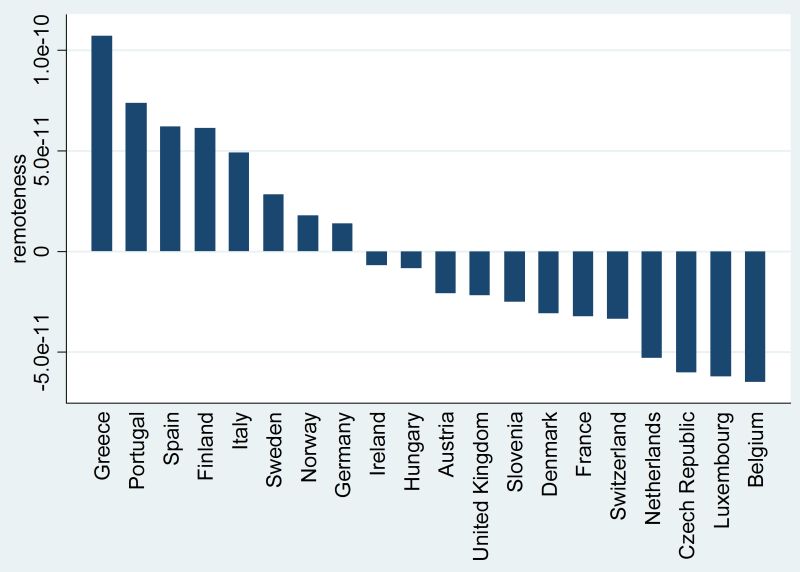
Remoteness comparison across countries.

Figure 1: Remoteness comparison across countries.

Equations (iv), (v), (vi) in Table 1 are estimated by restricting the dataset to 1995, 2000 and 2005 respectively. All estimates are quite consistent and do not exhibit much variation across time. Chow structural change test ^[3] shows that we cannot reject the hypothesis that slope coefficients in models (iv), (v), (vi) are different from model (iii). Moreover, we cannot reject the hypothesis that coefficients on home are statistically different from each other. In model (vii) we restrict slope coefficients to be constant over time; however, we allow for dynamics in the home coefficient by including interactive dummies. On average countries traded 0.93% and 0.89% more in 2000 and 2005 respectively compared to 1995 (adjusted for inflation). The negative and statistically significant estimates on t2 x Home and t3 x Home suggest that border effects among European Union countries decrease over time. A Wald test shows that the implied average border effect of 10.08 in 1995 is statistically different from 6.81 ^[4] and 5.79 ^[5], the border effects in 2000 and 2005. The sample comprises 20 European countries, most of which are members of the European Union, so it is not surprising that these countries have become more economically integrated and that they now trade more with each other relative to domestic trade. However, the statistical test indicates that the rate of the border effect decline has been decreasing over time: we cannot reject the hypothesis that average border effects on trade in 2000 and 2005 are equal to each other.^[6]

To investigate the dynamics of border effects further, our sample of countries was split into three groups: countries that founded the European Union ('old members': Germany, France, Italy, Luxembourg, Belgium and Netherlands), countries that joined EU from then until 2004 ('medium group') and the ones that joined in 2004 ('new members': Czech Republic, Hungary and Slovenia). Estimated border effects for these three groups of countries are reported in Figure 2. There is no variation in border effects for the group of old EU members. 'Medium' group countries on average have border effects that closely match the average of the whole sample. Border effects in the most recent members of the union have dropped sharply since 1995. The reason for this phenomenon is that countries started preparing for the accession and adopted many EU policies before 2004 so the integration began before the actual accession.

The assessment of EU policies is ambivalent. On the one hand, the convergence of border effects shows a successful implementation of EU policies in the new member countries. On the other hand, old member countries do not benefit that much. The expansion of the union does not encourage them to trade more with other countries relative to their domestic trade. The reason for that might be the smaller size of the new members. The combined GDP (in real terms) of the Czech Republic, Hungary and Slovenia is only about 7% of that of Germany, which is the biggest EU country. Finally, although the convergence means that the union is getting more integrated, the estimated border effect in 2005 for the whole EU is still about 6; there is still much to be done in order to achieve perfect market integration and full openness amongst EU countries.

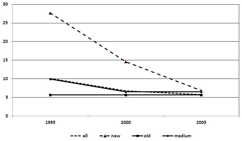
Figure 2: Border Effects within the EU

Figure 2: Border Effects within the EU

Sensitivity to domestic distances

Many papers claim that border effect estimates are quite sensitive to a chosen method of measuring domestic distances (see Head and Mayer, 2002; Nitzch, 2000: 1096; Chen, 2004: 112-14). If a higher value for domestic distance is assigned to each country, then the difference between the distances of domestic trade and international trade narrows; the home bias in trade becomes higher. We expect to find a positive relationship between the domestic distances and border effects. Some sensitivity tests have been performed to check this. The model (i) in Table 3 uses Leamer's (1997) proposed domestic distances. They are calculated by representing a country's geographic area as a circle with the economic centre of the country in the centre of that circle. Domestic distance is equal to the radius of that circle. In (ii) we use two thirds of that radius as a proxy for domestic distances (Head and Mayer, 2000: 294). They represent the economic centre in the centre of the circle and consumers spread around uniformly. Domestic distances in (iii) are computed by a formula 0.52√area (Helliwell and Verdier, 2001: 1034) and in (iv) they are a half of a distance from a capital to the closest border (Wei, 1996: 27-28). Our results confirm the hypothesis of the sensitivity of border effect estimates: the coefficients on home vary substantially. We reach a conclusion that border effects and the domestic distance measure are highly correlated: the greater the average domestic distances, the higher the border effect.

Eq no.	(i)	(ii)	(iii)	(iv)
Dependant variable	ln(trade_ij) 1995,2000,2005	ln(trade_ij) 1995,2000,2005	ln(trade_ij) 1995,2000,2005	ln(trade_ij) 1995,2000,2005
constant	-30.407*** (11.049)	-30.407*** (11.049)	-30.407*** (11.049)	12.016 (11.107)
ln(distance_ij)	-1.318*** (0.058)	-1.318*** (0.058)	-1.318*** (0.058)	-1.110*** (0.061)
ln(remoteness_ij)	-1.648*** (0.362)	-1.648*** (0.362)	-1.648*** (0.362)	-0.685* (0.375)
ln(remoteness_ji)	-0.742** (0.362)	-0.742** (0.362)	-0.742** (0.362)	0.212 (0.375)
Adjacency	0.389*** (0.064)	0.389*** (0.064)	0.389*** (0.064)	0.494*** (0.068)
Home	2.000*** (0.149)	1.472*** (0.169)	1.892*** (0.152)	1.505*** (0.201)
Border effect	7.39	4.36	6.63	4.50
Adjusted R²	0.937	0.937	0.937	0.928
Average domestic distance	213.30	142.91	196.59	90.20
Comments:	Fixed Effects, Leamer distances	Fixed Effects, Head and Mayer distances	Fixed Effects, Helliwell and Verdier distances	Fixed Effects, Wei distances

Table 2: Sensitivity of border effects to domestic distances.
*, ** and *** indicate significance at respectively 10%, 5% and 1%.

Leamer distances were used in our analysis of border effects. If, for example, Head and Mayer distances had been used instead, much smaller border effects would have been estimated. The difference might be up to 50%.^[7]

Nationalism and border effects

A potential cause of border effect might be consumer preferences. If consumers have a preference for domestic goods then there would be more goods traded domestically. Evans (2003) links consumer preferences and border effects; she collects data on sales of US companies producing in foreign countries. Then she compares imports from US with the sales of the US foreign affiliates, and also US foreign affiliate sales to domestic sales. The former allows examining 'location effect' - that is, the importance of the place where a product has come from - while the latter controls for location and shows 'nationality effect'. Evans discovers that the location of the source of goods plays a more important role in explaining the economic significance of borders. However, her method suffers from a major flaw: once a company produces goods in a foreign country, the final product there might be different from the one produced in the home country and more similar to other foreign country products. This happens because of potentially different production processes and inputs used. When a US company establishes a foreign affiliate in Europe, it might also change some product features in order to meet the preferences of local consumers.

Marketing literature has addressed the issue of domestic country bias in consumer preferences. Quite a few micro-level studies investigate country-of-origin and consumer ethnocentrism effects on consumer behaviour (see Bilkey and Nes, 1982, and Sammie, 1994, for good literature surveys). Balabanis and Diamantopoulos (2004) confirm that, although not entirely consistent across different product groups, ethnocentrism is positively related with preferences for domestic goods and negatively related with preferences for foreign goods. As Balabanis et al. (2001) find a positive nationalism relationship to consumer ethnocentrism, we predict that the border effect puzzle can be explained, at least partially, by the differences in nationalism.

H1: More nationalistic countries have larger border effects.

We approximate nationalism by four different variables. Variable 'very close' is taken from the International Social Survey 2003. There is a question asking how closely related respondents feel with their home country. The variable is composed as a proportion of respondents in the sample who chose the top answer, 'very close'. Similarly, the variable 'close' was generated by those individuals who picked both the first and the second highest answers. The next variable we use is a proportion of seats in parliament taken by right-wing parties. According to the standard political spectrum theory those parties should favour more nationalistic ideas and the fact that people have voted for them might also approximate how nationalistic a country is. The last nationalism variable is also taken from the International Social Survey 2003. It is a proportion of respondents, who claim that it is very important to feel British, German, or other nationality that they were with.

Eq no.	(i)	(ii)	(iii)	(iv)
Dependant variable	Ln(trade_ij) 1995,2000,2005	Ln(trade_ij) 1995,2000,2005	Ln(trade_ij) 1995,2000,2005	Ln(trade_ij) 1995,2000,2005
Constant	-47.537*** (12.085)	-61.840*** (11.969)	-30.407*** (11.049)	-46.683*** (11.987)
ln(distance_ij)	-1.359*** (0.066)	-1.347*** (0.064)	-1.318*** (0.058)	-1.379*** (0.066)
ln(remoteness_ij)	-1.859*** (0.397)	-2.171*** (0.390)	-1.644*** (0.362)	-1.846*** (0.395)
ln(remoteness_ji)	-1.289*** (0.393)	-1.596*** (0.387)	-0.738** (0.362)	-1.270*** (0.391)
Adjacency	0.414*** (0.073)	0.460*** (0.072)	0.389*** (0.064)	0.394*** (0.073)
Home	0.175 (0.407)	-11.879*** (1.727)	2.056*** (0.296)	-0.356 (0.482)
Home x N	3.536*** (0.761)	15.239*** (1.900)	-0.116 (0.522)	4.266*** (0.854)
N=	How close do you feel to your country? 'very close'	How close do you feel to your country? 'very close'+ 'close'	'proportion of parliament seats taken by right wing parties '	How important to feel (nationality)? 'very important'
Mean of N	0.465	0.897	0.490	0.501
Border effect (at the mean of N)	6.17	5.99	7.38	8.44
Adjusted R²	0.929	0.932	0.937	0.929
Comments	Fixed Effects	Fixed Effects	Fixed Effects	Fixed Effects
Boundaries of BE when N [0,100]	[0,34.16]	[0,28.78]	[7.38,7.38]	[0,50]

Table 3: Nationalism and border effects.
*, ** and *** indicate significance at respectively 10%, 5% and 1%.

Table 3 reports how border effects vary with a prevalence of nationalism in the exporting country. The direct effect of nationalism on the level of bilateral trade cannot be estimated with fixed effects. From (i) we observe that the multiplicative variable Homex very close is positive and statistically significant, while Home gets insignificant. This suggests that more nationalistic countries have a higher border effect. The variable predicts 0 border effect for a country that has no nationalistic people (who feel very close to their country) and border effect of 34.158 (exp[3.356+0.175] = 34.156) for a fully nationalistic country. When we define nationalism more broadly in (ii), the coefficient on Home becomes negative and significant; however, it is offset by a high coefficient on Home x close. In this case the border effect is bounded between 0 (exp[-11.879] = 0) and 28.78 (exp[15.239-11.879] =28.78). The result also supports the hypothesis that border effects are higher in more nationalistic countries.

The variable comprising a proportion of right-wing parliament seats makes no significant difference on the estimates (compare with Table 2 equation (iii)). The variable was generated by using the distribution of seats in parliament across political parties in 2011. Quite a significant time gap between other variables and a right-wing parliament seats variable might explain why it does not give any significant results. Alternatively, the parties were assigned to the right-wing group by their political declaration about their position in the political spectrum, from centre-right to extreme-right. The majority of right-wing parties in parliaments represent a temperate position and claim to follow centre-right philosophy. As a result, the strength of their support for nationalism is vague. This explains why we do not get significant results in (iii).

The last nationalism variable in (iv) explains the border-effect variation from 0, when nobody thinks it is very important to be nationalistic, to 50, when 100% of population claims it is very important to feel connection with their nation.

In conclusion, 3 out of 4 nationalism variables explain the variation in border effects. The positive sign on the coefficients allows us to accept hypothesis 1: more nationalistic countries have larger border effects.

Cultural differences

Linder et al. (2005) find that two countries that are more culturally different from each other trade more than a pair of culturally less different countries. Linder et al. argue that for a higher cultural distance foreign production costs are higher than trading costs, because operating in a foreign country requires closer interaction with the locals. For this reason, companies of more culturally different countries are more likely to export their goods than produce at the foreign market. Watson and Wright (2000) say that cultural differences among countries have an effect on consumer choice between domestic and foreign goods. Yoo and Donthu (2008) employ Hofstede's cultural dimensions measure in order to investigate how cultural differences affect consumer ethnocentrism. They find that four out of five cultural dimensions are related to consumer ethnocentrism. Given that a relationship between preferences for domestic goods and cultural differences exists, we expect cultural differences to explain border effects. As stronger preference for domestic goods by definition would imply higher border effects, we expect the sign of the cultural differences effect on border effects to be the same as that of the cultural differences effect on the consumer ethnocentrism. As a result, based on Yoo and Donthu's (2008) findings, we predict that:

H2: Power Distance is related positively to border effects.

H3: Individualism is related negatively to border effects.

H4: Masculinity is related positively to border effects.

H5: Uncertainty avoidance is related positively to border effects.

H6: Long-term orientation is related negatively to border effects.

H7: Indulgence is related negatively to border effects.

The same cultural dimension indicators developed by Hofstede (1994) are used in our analysis. The dimensions quantify the cultural differences between countries by assigning each of them a score from 1 to 100 in six different categories: power distance, individualism, masculinity, uncertainty avoidance, long-term orientation and social restrain. For more detailed descriptions of the dimensions see Appendix 3.

The dimensions of the exporting country were included in our regression in order to see which cultural aspects have an impact on trade patterns (Table 4). In our results they are defined as a deviation from the mean of the sample of 20 countries. We find that countries that have a higher score in individualism, long-term orientation and indulgence dimensions have lower border effects; a higher score in the power distance and uncertainty avoidance dimensions imply higher border effects. The evidence supports hypotheses 2, 3, 5, 6 and 7. The hypothesis number 4 is not supported as the interaction term on masculinity variable is not statistically significant. However, masculinity dimension has a negative effect on the general trade volume: societies defined as more feminine (see Appendix 3) trade more compared to those defined as more masculine.

To sum up, we have found a relationship between cultural differences and border effects.

Eq no.	(i)	(ii)	(iii)	(iv)	(v)	(vi)
Dependant variable	ln(trade_ij) 1995,2000, 2005	ln(trade_ij) 1995,2000, 2005	ln(trade_ij) 1995,2000, 2005	ln(trade_ij) 1995,2000, 2005	ln(trade_ij) 1995,2000, 2005	ln(trade_ij) 1995,2000, 2005
Constant	-25.893** (10.851)	-39.078*** (11.064)	-30.317*** (11.046)	-26.706** (10.975)	-33.318** (10.587)	-31.540*** (11.259)
ln(distance_ij)	-1.291*** (0.057)	-1.261*** (0.058)	-1.321*** (0.058)	-1.276*** (0.058)	-1.310*** (0.058)	-1.304*** (0.058)
ln(remoteness_ij)	-1.563*** (0.357)	-1.711*** (0.356)	-1.690*** (0.363)	-1.587*** (0.356)	-1.724*** (0.363)	-1.587*** (0.359)
ln(remoteness_ji)	-0.657* (0.357)	-0.809** (0.356)	-0.784** (0.363)	-0.683** (0.356)	-0.818** (0.363)	-0.682** (0.358)
Adjacency	0.397*** (0.063)	0.440*** (0.064)	0.388*** (0.064)	0.420*** (0.063)	0.396*** (0.064)	0.398*** (0.063)
Home	2.069*** (0.147)	2.058*** (0.147)	1.987*** (0.149)	2.098*** (0.147)	1.967*** (0.149)	1.996*** (0.147)
Home x Dimension	0.026*** (0.004)	-0.027*** (0.005)	-0.005 (0.003)	0.017*** (0.003)	-0.012** (0.005)	-0.023*** (0.005)
Dimension name	Power distance	Individualism	Masculinity/Femininity	Uncertainty Avoidance	Long Term Orientation	Indulgence
Mean of N	43.55	63.3	46.45	67.4	54.4	52.85
Border effect (at the mean Dimension)	8.00	7.91	7.15	7.68	6.98	7.36
Adjusted R	0.939	0.939	0.936	0.939	0.937	0.937
Fixed Effects	Yes	Yes	Yes	Yes	Yes	Yes
Boundaries of BE when dimension [0,100]	[7.9;106.6]	[0;7.8]	[4.4;7.3]	[8.1;44.6]	[2.1;7.1]	[0;7.4]

Table 4: Cultural differences.
*, ** and *** indicates significance at respectively 10%, 5% and 1%

Endogeneity discussion

Our estimated models show a relationship between nationalism and border effects as well as cultural differences and border effects. To claim a true causal effect we need to be sure that there is no other force that has an impact on these factors and also has an effect on border effects. A possible candidate is non-tariff barriers. There are no tariffs between our sample countries but more nationalistic countries favouring their domestic producers might impose some bureaucratic regulations that make trading with other countries more complicated. However, as well as zero tariffs, the EU has a number of common health and safety and quality standardisation policies in place suggesting that the countries have a small number of ways to control international trade in favour of domestic producers. To investigate this we compared our nationalism variables against the 2005 values of a regulatory-trade barriers index (Gwartney et al., 2011: 7-8). This assesses non-regulatory barriers and the compliance costs of exporting and importing. The correlation between all our nationalism, cultural differences variables and the index is quite weak (see Appendix 2 for covariance matrix); the evidence does not show higher regulatory barriers in the countries which have a higher prevalence of nationalism. Furthermore, Chen (2004: 101-02), analysing industry-level border effects in seven Western European economies, finds no significant evidence that non-tariff barriers explain border effects on trade.

It is more complicated to make conclusions about the relationship between consumer preferences and border effects. As explained above, other authors have found a causal relationship between nationalism and consumer preferences. We have established a relationship between national identity variables and border effect. The direction of the effects matches the hypothesis that consumers have a preference for domestic goods and it explains border effects. However, preferences are determined by many other factors for which our model does not control. The factors might amplify, reduce or even completely change the true effect. For this reason our evidence in the support of consumer preferences and border effect relationship might be weak.

Conclusion

We calculated border effects for a sample of European Union countries. The average border effect is approximately 7.5, although the domestic distance analysis suggests that our estimates are elevated. The analysis of different EU member groups revealed a rapid decrease in border effects for countries that joined the union in 2004, a marginal decrease for 'medium' group countries and no variation for the old member-countries, i.e. founders of the union. The convergence of the border effects implies that EU policies and regulation boost trade among its members.

This article proposed a new approach to the border effect puzzle: to investigate consumer preferences. In order to find a relationship between border effects and consumer preferences, we used variables for nationalism and cultural differences. We have shown that nationalism and most of the cultural dimensions explain a great deal of variation in border effects. The findings suggest that consumer preference heterogeneity is an important reason why we observe border effects in international trade. This finding indicates that no trade-related policy can eliminate border effects, because they are the result of consumers' optimal choice of the products they like. Combined together our results imply that high estimates of border effects arise because of two distinct reasons: trade frictions, which, as European Union example shows, can be eliminated by correct trade policies and economic integration; and optimal consumer choice. So, following this idea, we would expect to estimate a low (but existent) border effects in a frictionless but culturally segregated market.

The difficulty of modelling consumer preferences poses the main challenge to this research. We believe that the variables that we used approximate the preferences reasonably well. However, validating this statement empirically is very challenging. More advanced structural estimation is needed in order to establish a strong link between consumer preferences and the cultural variables and nationalism. We believe that such research should focus on a product-specific or product-group-specific dataset and then aggregate the estimates across a high number of products. This approach, although very data intensive, would eliminate the 'noise' of the aggregated bilateral trade data. Moreover, it would allow for more detailed investigation of the mechanism how each specific cultural and nationalistic feature influences trade patterns

Acknowledgements

The author is grateful to Professor Kimberley Scharf for her supervision and guidance; to Professor Natalie Chen for her invaluable thoughts and discussion; and to the anonymous reviewers for their comments.

List of figures

Figure 1: Remoteness comparison across countries

Figure 2: Border effects within the EU

List of tables

Table 1: Border effects

Table 2: Sensitivity of border effects to domestic distances

Table 3: Nationalism and border effects

Table 4: Cultural differences

Appendices

Appendix 1: data

Country list

Austria
Belgium
Czech Republic
Denmark
Finland
France
Germany
Greece
Hungary
Ireland
Italy
Luxembourg
Netherlands
Norway
Portugal
Slovenia
Spain
Sweden
Switzerland
United Kingdom

Variables

International trade flows. The variable indicates the value of goods shipped from one country to another. Services are assumed to be non-tradable and therefore excluded from the analysis. Values are expressed in US dollars (PPP adjusted) and adjusted for inflation.

Domestic trade flows are estimated using the formula:

trade_ii = total production_i - total export of goods_i

Data for the total production was collected from the OECD input-output database. Total production variable covers industries coded from 1 to 45 (ISIC Revision 3).

GDP. The variable is expressed in PPP US dollars and adjusted for inflation. Data source: World Development Indicators, The World Bank.

Remoteness. The variable is defined as

$remoteness_{i} = \Bigg(\sum_{j,j\neq{i}}\frac{GDP_j}{distance_{ij}}\Bigg)^{-1}$

International distances. A measure of distance between two countries is calculated as a distance between two capital cities. We collected data for geographic coordinates of capitals ^[8] and then applied Hiversine formula to calculate distances in kilometres.

Appendix 2: regulatory trading barriers

Correlation coefficients between regulatory trade barriers index and nationalism variables.

	Regulatory Trade Barriers
How close do you feel to your country? 'very close'	-0.061
How close do you feel to your country? 'very close' + 'close'	-0.284
'proportion of parliament seats taken by right wing parties'	-0.154
How important to feel (nationality)? 'very important'	0.054

Appendix 3: cultural dimensions

Cultural dimensions, as Hofstede (1994)^[9] defined them:

Dimension 1: Power distance

This is the extent to which the less powerful members of organisations and institutions (such as the family) accept and expect that power is distributed unequally. This represents inequality (more versus less), but defined from below, not from above. It suggests that a society's level of inequality is endorsed by the followers as much as by the leaders.

Dimension 2: Individualism

Individualism on the one side versus its opposite, collectivism, is the degree to which individuals are integrated into groups. On the individualist side, we find societies in which the ties between individuals are loose: everyone is expected to look after him/herself and his/her immediate family. On the collectivist side, we find societies in which people from birth onwards are integrated into strong, cohesive in-groups, often extended families (with uncles, aunts and grandparents) which continue protecting them in exchange for unquestioning loyalty.

Dimension 3: Masculinity versus Femininity

Masculinity versus its opposite, femininity, refers to the distribution of roles between the sexes which is another fundamental issue for any society to which a range of solutions are found. The IBM studies revealed that: (a) women's values differ less among societies than men's values; (b) men's values from one country to another contain a dimension from very assertive and competitive and maximally different from women's values on the one side, to modest and caring and similar to women's values on the other. The assertive pole has been called 'masculine' and the modest, caring pole 'feminine'. The women in feminine countries have the same modest, caring values as the men; in the masculine countries they are somewhat assertive and competitive, but not as much as the men, so that these countries show a gap between men's values and women's values.

Dimension 4: Uncertainty Avoidance

Uncertainty avoidance as a fourth dimension was found in the IBM studies and in one of the two student studies. It deals with a society's tolerance for uncertainty and ambiguity: it ultimately refers to person's search for truth. It indicates to what extent a culture programs its members to feel either uncomfortable or comfortable in unstructured situations. Unstructured situations are novel, unknown, surprising and different from usual. Uncertainty avoiding cultures try to minimise the possibility of such situations by strict laws and rules, safety and security measures, and on the philosophical and religious level by a belief in absolute truth; 'there can only be one truth and we have it'. People in uncertainty-avoiding countries are also more emotional, and motivated by inner nervous energy. The opposite type, uncertainty-accepting cultures, are more tolerant of opinions which are different from those they are used to; they try to have as few rules as possible, and on the philosophical and religious level they are relativist and allow many currents to flow side by side. People within these cultures are more phlegmatic and contemplative, and not expected by their environment to express emotions.

Dimension 5: Long-Term versus Short-term Orientation

This fifth dimension was found in a study among students in 23 countries around the world, using a questionnaire designed by Chinese scholars (The Chinese Culture Connection, 1987). It can be said to deal with Virtue regardless of Truth. Values associated with long term orientation are thrift and perseverance; values associated with short term orientation are respect for tradition, fulfilling social obligations, and protecting one's 'face'.

Dimension 6 - Indulgence versus restraint

Indulgence stands for a society that allows relatively free gratification of basic and natural human drives related to enjoying life and having fun. Restraint stands for a society that suppresses gratification of needs and regulates it by means of strict social norms.

Notes

[1] Originally from Lithuania, Mantas Vanagas completed a BSc in Economics at the University of Warwick in 2012 and then went on to study for an MPhil in Economics in Cambridge, where he had a keen interest in macroeconomic forecasting. He has now started working in economic research in the City of London.

[2] Germany, the most open European economy, is the only exception. The way distances are measured explains the 'remoteness' of Germany. The distance between two countries is approximated by the distance between capital cities; as Berlin is located in the north-east part of Germany and the country is quite large in terms of land area, the distance from the capital to other capital cities of major European economies is quite big, despite the fact that Germany is quite central.

[3] Test statistics F=1.29 is smaller than a critical value F(0.05, 12, 1116) = 1.7522

[4] Test statistics F=4.42 is larger than a critical value F(0.05, 1, 995) = 3.841

[5] Test statistics F=8.55 is larger than a critical value F(0.05, 1, 995) = 3.841

[6] Test statistics F=0.730 is smaller than a critical value F(0.05, 1, 995) = 3.841

[7] Calculated taking the percentage difference between the highest and the smallest Home coefficients in table 3 and applying to the highest home coefficient, 2.62, in table 2, because border effect is an exponential function of the home coefficient. 1 - {exp[(1.472/2) x 2.62]/ exp[2.62]}=0.50

[8] Source: http://www.timegenie.com/latitude_and_longitude/

[9] The paper does not talk about a dimension number 6 'Indulgence vs. Restraint' as it was developed later. The description of the dimension 6 is taken from Hofstede's person website: http://geert-hofstede.com/national-culture.html

References

Anderson, J. E. and E. van Wincoop (2003), 'Gravity in Gravitas: A solution to the Border Puzzle', The American Economic Review, 93 (1), 170-92

Balabanis, G. and A. Diamantopoulos (2004), 'Domestic country bias, country-of-origin effects, and consumer ethnocentrism: A multidimensional unfolding approach', Journal of the Academy of Marketing Science, 32 (1), 80-95

Balabanis, G., A. Diamantopoulos, R. D. Mueller and T. C. Melewar (2001), 'The Impact of Nationalism, Patriotism and Internationalism on Consumer Ethnocentric Tendencies', Journal of International Business Studies, 32 (1), 157-75

Bilkey, W. J. and E. Nes (1982), 'Country-of-Origin Effects on Product Evaluations', Journal of International Business Studies, 13 (1), 89-99

Chen, N., (2004), 'Intra-national versus international trade in the European Union: Why do national borders matter?', Journal of International Economics, 63, 93-118

Crucini, M. J., C. I. Telmer and M. Zachariadis (2003), 'Price Dispersion: The Role of Borders, Distance and Location', Tepper School of Business, paper 490

Engel, C. and J. H. Rogers (2001), 'Deviations from purchasing power parity: causes and welfare costs', Journal of International Economics, 55, 29-57

Evans, C. L. (2003), 'The Economic Significance of National Border Effects', The American Economic Review, 93 (4), 1291-312

Head, K. and T. Mayer (2000), 'Non-Europe: The Magnitude and Causes of Market Fragmentation in Europe', Weltwirtshcaftliches Archiv, 136 (2), 285-314

Head, K., and T. Mayer (2002), 'Illusory Border Effects: Distance mismeasurement inflates estimates of home bias in trade', Paris: CEPII research center

Helliwell, J. F. (1997), 'National Borders, trade and migration', National Bureau of Economic Research, Working Paper 5215

Helliwell, J. F. and G. Verdier (2001), 'Measuring internal trade distances: a new method applied to estimate provincial border effects in Canada', Canadian Journal of Economics, 34 (4), 1024-41

Hillberry, R. (1999), 'Explaining the "border effect": what can we learn from disaggregated commodity flow data?', Indiana University Graduate Student Economics Working Paper Series 9802, Indiana University

Hofstede, G. (1994), 'The business of international business is culture', International Business Review, 3 (1), 1-14

Gwartney, J., J. Hall and R. Lawson (2011), 'Economic Freedom of the World: 2010 Annual Report', Economic Freedom Network

Leamer, E. E. (1997), 'Access to western markets, and eastern effort levels', In Zecchini, S. (ed.), Lessons from the Economic Transition: Central and Eastern Europe in the 1990s, Dordrecht and Boston: Kluwer Academic Publishers, pp. 503-26

McCallum, J. (1995), 'National Borders matter: Canada-US regional trade patterns', American Economic Review, 85 (3), 615-23

Nitsch, V. (2000), 'National Borders and International Trade: Evidence from European Union', Canadian Journal of Economics, 33 (4), 1091-105

Obsfeld, M. and K. Roggoff (2000), 'The six major puzzles in International Macroeconomics: Is there a common cause?', National Bureau of Economics Research Paper 7777

Samiee, S. (1994), 'Customer Evaluation of Products in a Global Market', Journal of International Business Studies, 25 (3), 579-604

Shimp, T. A. and S. Sharma 'Consumer Ethnocentrism: Construction and Validation of the CETSCALE', Journal of Marketing Research, 24 (3), 280-89

Wei, S. J. (1996), 'Intra-national versus international trade: how stubborn are nations in global integration?', National Bureau of Economics Research Working Paper 5531

Wolf, H. (2000), 'International Home bias in trade', The Review of Economics and Statistics, 82 (4), 555-63

Watson, J. J. and K. Wright (2000), 'Consumer ethnocentrism and attitudes toward domestic and foreign products', European Journal of Marketing, 34 (9), 1149-66

Yoo, B. and N. Donthu (2005), 'The Effect of Personal Cultural Orientation on Consumer Ethnocentrism', Journal of International Consumer Marketing, 18 (1), 7-44

To cite this paper please use the following details: Vanagas, M. (2013), 'Border Effects Among EU Countries: Do National Identity and Cultural Differences Matter?', Reinvention: an International Journal of Undergraduate Research, Volume 6, Issue 2, http://www.warwick.ac.uk/reinventionjournal/issues/volume6issue2/vanagas Date accessed [insert date]. If you cite this article or use it in any teaching or other related activities please let us know by e-mailing us at Reinventionjournal at warwick dot ac dot uk.