
2D Simulation
Rescaling the domain
In order to run the Barkley model such that spirals are produced on a general square domain, some rescaling is necessary. For convenience, define \( \Omega_c \) for \( c \in \mathbb R ^+ \) to be the interval \( [0,c ]^2 \).
We know that the Barkley equation with parameters
\begin{equation*} \Gamma =\Omega_{150} , ~~ \epsilon = {1 \over {50}}, ~~ a=1, ~~b= {1 \over {100} } ~~c={3 \over 4 } \end{equation*}
and initial conditions
\begin{equation*} u_0 = \mathbb I _{ {y \over {150}} > {{51} \over {100}}} , ~~ v_0 = \mathbb I _{ {y \over {150}} > {{51} \over {100}}} \end{equation*}
gives a spiral \( u: \Omega_{150} \to [0,1] \) when evaluated using the finite difference method. Now, we want to change the domain of \( u \). We can rescale to \( \Omega _L \) so that we have an equation for \( \tilde u , \tilde v : \Omega_L \to [0,1] \) where
\begin{align*} \tilde u (t,x) &= u \left( t , {{150} \over {L}} x \right) \\ \tilde v (t,x) &= v \left( t , {{150} \over {L}} x \right) \end{align*}
which are solutions to the rescaled Barkley equation
\begin{align*} \partial_t \tilde u- { {L^2} \over {150^2}} \Delta \tilde u &=f \left( \tilde u, \tilde v \right) \\ \partial_t \tilde v &= g \left( \tilde u,\tilde v \right) \end{align*}
where we have chosen the appropriate time derivative and Laplace-Beltrami operator for our problem and recalled that \( \mathbf{v} \equiv 0\) as the surface is stationary.
Stability of the 2D scheme
Ultimately, we wish to simulate spiral waves on a unit sphere. The surface area of a unit sphere is \( 4 \pi \). We want our spherical domain and square domain to have the same area. The area of a square is \( L^2 \) so we require
\begin{equation*} L^2= 4 \pi \end{equation*}
which implies that our square domain is \( \Omega_{3.5} \) (since \(L = \sqrt{2 \pi} \approx 3.5\) ). From the calculations above, a reasonable value of the diffusion coefficient \(a \) is
\begin{align*} a &= { {4 \pi } \over { 150^2 }} \\ & \approx {1 \over {1790.49}} \end{align*}
Unfortunately this does not give us stable results, so we change the coefficient to be
\begin{align*} a &= {1 \over {179.049}}, \end{align*}
which does provide stability.
We also tested
\begin{equation*} a= {2 \over {1790.49}} , {1 \over {500}} , {1 \over {350}} , {1 \over {250}} \end{equation*}
all of which produced instability.
Finite element versus finite difference
We know that we can obtain results using both a semi-implicit method and an explicit method. We are also able to compute results using the finite differences method. In this case the numerical scheme can be again given as a \(\theta \) scheme with explicit left hand-side
\begin{equation*} u^{n+1} -a \tau \theta {\Delta_ \Gamma }^ h u^{n+1} =\left( 1-\theta \right) a \tau{\Delta_ \Gamma }^ h u^n + u^n + \tau f \left(u^n , v^n \right) \end{equation*}
where \( u^n \) is defined on a finite spatial grid \( u^n =u^n (i,j,k) \) and thus
\begin{equation*} {\Delta_ \Gamma }^ h u^n (i,j,k ) = \partial_x^2 u^n (i ,j,k) + \partial_y^2 u^n (i ,j,k) \end{equation*}
where
\begin{equation*} \partial_x^2 u^n (i ,j,k) ={{u^n (i+1,j,k ) -4 u^n(i,j,k) + u^n(i-1,j,k ) }\over {h^2}} \end{equation*}
using the forward diference and backward difference
\begin{align*} \partial_{x+} u^n (i,j,k ) & = {{ u^n(i+1,j,k) - u^n (i,j,k) } \over {h_x}}\\ \partial_{x-} u^n (i,j,k ) & = {{ u^n(i,j,k) - u^n (i-1,j,k) } \over {h}} \end{align*}
and that
\begin{equation*} \partial_x^2 u^n (i,j,k) = \partial_{x+} \partial_{x-}u^n (i,j,k) \end{equation*}
and \( \partial_y u^n \) is defined similarly
The numerical scheme can also be given as in a semi-implicit form. If we define
\begin{equation*} u_{th} = {{v^n +b } \over c} \end{equation*}
Then our equation is:
\begin{cases} \left( 1+ \tau \epsilon \left( 1- u^n \right) \left( u_{th} -u^n \right) \right) u^{n+1}- a \tau {\Delta_ \Gamma }^ h u^{n+1} =u^n ~~~~~~~~~~~~~~~~~~~~~~~~ u_{th} \ge u^n \\ \left( 1 -\tau \epsilon \left( u_{th} -u^n \right) \right) u^{n+1} - a \tau {\Delta_ \Gamma }^ h u^{n+1} =u^n - \tau \left( u_{th} -u^n \right) u^n ~~~~~~~~~ u_{th} \le u^n \end{cases}
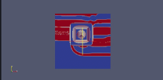
Tests on \(\Omega_{3.5}\) with \(a=\frac{1}{1790.49}\), time=10
Top left: using FD explicit RHS method.
Top right: using FEM explicit RHS method.
Bottom left: using FD semi-implicit RHS method
Bottom right: using FEM semi-implicit RHS method.
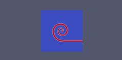
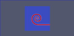
Spiral on a \(\Omega_{3.5}\), \(a=1/1790.49\).
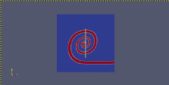
Spiral on a \(\Omega_{3.5}\), \(a=1/179.049\).