Metal 'n' Roll

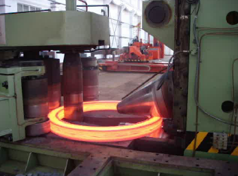Ring Rolling in action Our project looked into metal ring rolling. Ring rolling is a forming process in metal industry to shape a metal workpiece into a final product by repeatedly passing a steel ring between two vertical rolls. Although ring rolling is used a lot, e.g. for oil platform legs or aircraft engine parts, a flexible and accurate analytical model does not exist. As such a model is desired; not only could it lead to further automation, it could also allow more control over the ring profile, saving energy and material. We followed an approach began by Jeremy Minton, splitting the model into two parts, one for the roll gap region and one for the outer region.

Inner Model

$x^n_t$ and $x^n_b$ refer to the neutral points on the top and bottom roll respectively: these are 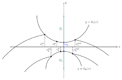Inner Model Diagram points at which the direction of friction changes, so that material is pushed towards neutral points.

$h_t(x)$ and $h_b(x)$ parametrize the top and the bottom roll respectively.

We denote with
$\mathbf{\sigma} = \begin{pmatrix} \sigma_x & \tau \\ \tau & \sigma_y \end{pmatrix}$
the stress tensor within the roll gap.

Slab Analysis

Based on a force and moment balance along each small vertical strip between the rolls we derive the following equations.
$\partial_x & \int_{h_b}^{h_t} \sigma_x \, y \, dy = \int_{h_b}^{h_t} \tau \, dy + h_t(h_t'\sigma_t -\tau_t) -h_b(h_b'\sigma_b - \tau_b)$

$\partial_x & \int_{h_b}^{h_t} \tau\,dy = h_t'\tau_t -h_b'\tau_b - \sigma_y(h_t) + \sigma_y(h_b)$

$\partial_x & \int_{h_b}^{h_t} \sigma_x \, dy = h_t'\sigma_t - \tau_t - h_b'\sigma_b + \tau_b$

where we abbreviate $\sigma_t = \sigma_x(h_t)$ and $\sigma_b = \sigma_x(h_b)$ , as well as $\tau_t = \tau(h_t)$ and $\tau_b=\tau(h_b)$ . In order to get a problem which is neither underconstrained nor overconstrained, we assume the the following yield condition which refers to plastic deformation
$\left(\frac{\sigma_x - \sigma_y}{2}\right)^2 + \tau^2 = k^2$
where $k$ is a material constant. Moreover, we make use of a friction law at the top and bottom, where the workpiece contacts the roller and we assume that the horizontal stress varies linearly through the
thickness
$\sigma_x(y) = \frac{\sigma_t - \sigma_b}{\Delta h}y+\frac{\sigma_bh_t- \sigma_th_b}{\Delta h}$
where $\Delta h = h_t - h_b$ .

Outer Model

The outer model aims to predict the behaviour of the beam outside the roll gap.
The forces on this part of the beam are much smaller, so we model it as a curved beam undergoing elastic deformation.
We can use Castigliano's theorem, which relates the strain energy and the displacement as follows:
$\frac{\partial U }{\partial F_x} = \delta x$
Where $U$ is the strain energy, $F_x$ the force in direction $x$ and $\delta x$ the displacement in said direction.
For a curved beam the following was derived by Timoshenko (1925)
$U = \int_\Gamma \frac{M^2}{2 R A \gamma E} + \frac{S^2}{2AE} - \frac{MS}{AER} + \frac{\kappa Q^2}{2AG} ds<br />$ OuterModelResults
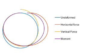
Here $M$ , $S$ , and $Q$ are the moment, longitudinal, and shear force respectively. We assume a force balance on each section of the beam to calculate them from an initial set of forces on one end, and $\Gamma$ parametrises the centreline of the beam. $\gamma$ , $R$ , $A$ , $\kappa$ , $E$ , and $G$ are functions or constants related to the beam. The figure shows some examples of a circular beam undergoing deformation from various forces.

Numerics

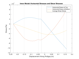
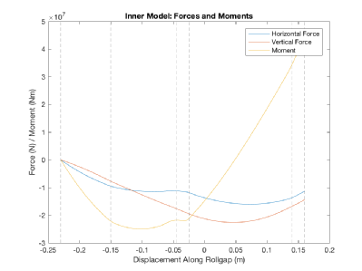
Below we plot the stress and force profiles in the inner model for two sets of parameters; in each case the left hand side shows the stresses and the right hand side the forces. In particular, the aspect ratio, i.e. the initial thickness of the workpiece divided by the length of the roll gap is changed.

Moderate Aspect Ratio

Small Aspect Ratio

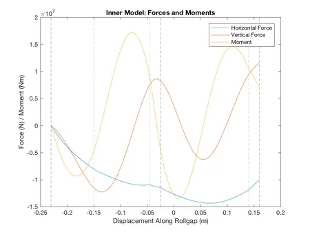
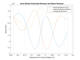
Small Aspect Ratio Forces Small Aspect Ratio Stress

As shown in the graphs, our model predicts large oscillations in the stresses when the roll gap is small. This is interesting but unverified, and could be due to numerical error in our model.

Report

Matlab Code

MATLAB Code

Please read the README.txt file for brief instruction on how to use our code. For further instructions, see the Numerics Appendix in our report.

Acknowledgements

We would like to thank our supervisors, Ed Brambley and Andreas Dedner, for all of their support. We also acknowledge ESPRC and MASDOC CDT funding that enabled us to carry out this project.

MASDOC

Warwick

EPSRC