
Jenkins et al. (2006)
Here you can find additional files associated with the paper "How many transcripts does it take to reconstruct the splice graph?" (Jenkins et al. 2006). Each file is described below. They are available together in this zip file.
ratios.xlscontains likelihood ratio tests for the pairwise versus in-out models applied to all 89 genes with more than 5000 putative transcripts, formatted as follows:
Region 1 ... Total all regions Ensembl ID Start of region (fragment number) End of region (fragment number) Gamma Degrees of freedom p-value (%)
readwg.mreads a directed ASG into Matlab. The ASG file should be formatted as in the exampleABCB5.wgand in the same directory.ABCB5.wgis an example weighted ASG file. ‘#’ acts as a comment character. Size of graph should be number of exon fragments + 2 (representing the appended source and sink). Below each node’s outdegree is a list of destination nodes and the supporting number of ESTs. There should also be a Y/N string indicating whether this node is attached to the next one (i.e. this and the following node are part of the same exon).pairwise.msimulates in Matlab the sampling of transcripts under the pairwise model as described in the paper. Execute this after reading in an ASG usingreadwg.m. It creates annx #exon-fragments matrix calledtranscripts(nis specified on input). Each row provides a random sample from the gene under the pairwise model.transcripts(i,j)is an indicator for whether exon fragment j is contained in sample i.inout.msimulates in Matlab the sampling of transcripts under the in-out model as described in the paper. It operates in the same way aspairwise.m.maxmin.mcreates variablesmaximum_transcriptsandminimum_transcriptswhich are the maximum and minimum number of informative transcripts obtainable from the current ASG. These values are calculated as described in the path-covering algorithms described in the paper. The current ASG is read into Matlab usingreadwg.m.ratio.mperforms the likelihood ratio test described in the paper on the current ASG, comparing the pairwise versus in-out models. It creates variablesregionstart,regionend,Gam,zandpvaluewhich are the rows of the table template above. The current ASG is read into Matlab usingreadwg.m. Determining the degrees of freedom under the pairwise model is not entirely straightforward. For a test on exons k,...,l we used the following as a sensible choice for the degrees of freedom under the pairwise model: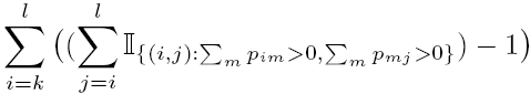
i.e. to describe all possible outgoing destinations from a given exon i we require the number of parameters to be equal to the number of downstream acceptor sites, minus 1. The degrees of freedom is the sum of all such i over k,...,l.putative_transcripts.mreturns the number of putative transcripts (i.e. distinct paths through the ASG) associated with the current ASG, which has been read into Matlab usingreadwg.m.count_downstream_paths.mis a function for use byputative_transcripts.m. Leave it in the same directory as this file.full_asg.pyis a Python script for which returns a p-value for an ASG, based on alpha = 1. Usage:
python full_asg.py m example.wg repeats
wheremis the number of transcripts we’ll draw for each repeat, andrepeatis the number of such repeats on which the p-value is based. This operates on the ASG contained inexample.wg. It should be executed in the same directory aswwdigraph.pyanddigraph.py, as well as yourexample.wg.