
Next Nearest Neighbour Interactions
In this section we work on the torus \(\Lambda=\{0,1,\dots,N+1\}\) and incorporating the tilt, consider Hamiltonians of the form
\begin{equation}
H_N(u_1, \ldots, u_N ) = \sum_{i=0}^N V \left(\frac{u_{i+1}-u_{i-1}}{2}+x\right).
\end{equation}
Theorem
For the pure next nearest neighbour model on the torus, assuming the potential \(V\) satisfies
\[ \forall \xi \in \mathbb R, \quad M(\xi)=\int_{\mathbb R} \exp( \xi y - \beta V(y) ) dy < \infty, \]and \(\exp(- \beta V) \in H^1( \mathbb R \backslash 0 )\), the limit behaviour of the free energy \(f_N\) is given by a Legendre transform,
\[ f(x)= F_\infty(x)-\frac1\beta \log 2z,\]
where
\[ F_\infty (x) := \frac 1\beta \sup_\xi \left( \xi x - \log \left[ z^{-1} M(\xi)\right] \right),\quad z=M(0). \]
The analysis of the free energy must be done in two cases, according to the parity of the number of atoms. (Note there are \(N+1\) atoms because we work on the torus \(\{0,1,\dots,N\}\).)
Even case:
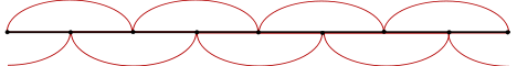
If \(N+1 = 2M\) then the model decomposes into two independent chains one containing all odd vertices and the other containing the even vertices.
Odd case:
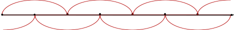
Alternatively, if \(N+1 = 2M+1\) then we have one chain containing all of the vertices.
In both cases one can reduce the calculations to those of the nearest neighbour model, with the only difference occurring from the increased distance between interacting particles.