
Mathematics of Multiscale Materials
Authors: Maha Al-Hajri, Tessa Colledge, Owen Daniel, Barnaby Garrod, Alexander Kister
Supervisors: Stefan Adams, Christoph Ortner
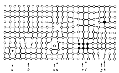
One goal of material science is to study the effects that microscopic defects have on the material on the macroscopic scale. Examples of such defects on the atomistic scale can be seen in Föll's image.
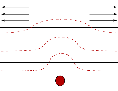
Studying such materials in realistic dimensions (i.e. \(d = 2, 3\) ) is typically hard, so we turn to a toy model in \(1\)-dimension which we hope captures some of the features of the material. To justify this approach we consider the model to be made up of many layers of particles, so that taking a cross section through the material results in a collection of \(1\)-dimensional systems stacked on top of one another, see figure below. The material could be under stress which is indicated by the arrows. The red dotted line represents the effect the deformation has on the layers.
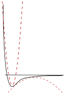
It is assumed that in this model the forces lead to a displacement of the atoms from the intial position and that displacements effect each other. In reality, the influence one atom has on a other atom at a distance \(r\) can be approximated reasonably well by the simple Lennard-Jones potential.
In physics interactions between many atoms can be modelled in the framework of statisctical mechanics. Since we are interested in displacements we choose the state space to be \(u\in\mathbb{R}^{\mathbb{Z}}\).
The Hamiltonians we consider are of the following type
\begin{equation} H_N(u) = \sum_{k=1}^K \sum_{\substack{i, j \in \Lambda \\ |i - j | = k }} V_k \left( \frac{u_i - u_j}{|i - j|} \right).\end{equation}
We may approximate Lennard-Jones by such potentials.
If \(K=1\) the models are called nearest neighbour models and for \(K=2\) they are called next nearest neighbour models. If \(K=2\) and additionally \(V_{1}=0 \) the models are called Pure Next-nearest neighbour models.
Nearest neighbour interactions
Acknowledgements
We acknowledge and thank the help of our supervisors.
We would also like to acknowledge the funding body EPSRC and the support from MASDOC CDT.