Spatial Lambda-Fleming-Viot Process
Click here to jump straight to the simulation animation below.
The Spatial \( \Lambda \)-Fleming-Viot process is a family of evolving random measures \((\rho_t(x)_{t \geq 0})_{x \in \mathbb{T}}\) on the type space E driven by a Poisson process \(\Pi = (t_i, x_i, r_i, u_i)_{i=1}^\infty\) on \([0,\infty)\times \mathbb{T} \times [0, \infty) \times [0,1]\) with intensity \(dt \otimes dx \otimes \mu(dr) \otimes \nu_r(du)\). Here they are indexed by points on a torus \(\mathbb{T}\), which we choose to avoid boundary conditions. At each event:
- We draw a parental location \(z_i \sim U(B_{x_i}(r_i))\) and a parental type \(\alpha_i \sim \rho_{t_i-}(z_i)\).
- We update each measure by \(\rho_{t_i}(y) \mapsto (1-u_i) \rho_{t_i-}(y) + u_i \delta_{\alpha_i} \) on the ball, and remain constant otherwise.
In order to simulate the process, we look at a finite particle system in order to approximate the measure through some form of empirical measure process. Here each lineage has a genetic type drawn from a finite space \(\{1, \dots, d\}). In this case, we update the process on the particles as follows. At each event:
- We still choose a parental location as before.
- We select \(u_i\) of the lineages in the ball and kill them off.
- The offspring genetic type is chosen according to a "lookdown" construction, which labels the lineages, and choses the type of the lowest-labelled lineage killed in the recolonisation-extinction event.
- A random number of offspring with this type (according to a fixed density) are placed uniformly in the ball.
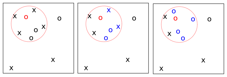
An extinction recolonisation event on the torus.
In addition to this, a mutation process runs alongside, where each lineage independently mutates according to a Poisson process with rate \(m>0\) according to a transition matrix \((P_{ \alpha \beta })\), with \( ( \gamma_{ \alpha } ) \) its stationary distribution.
Spatial \( \Lambda \)-Coalescent
The Spatial \( \Lambda \)-coalescent models the geneology of a finite collection of lineages backwards in time by extending \( \Pi \) to have events at times in \( \mathbb{R} \). Here each lineage has a genetic type drawn from a finite space \( \{1, \dots, d\} \). At each event backwards in time:
- We choose a \(u_i \) of lineages in \( B_{x_i}(r_i)\), restricting our choice to only subsets where all individuals are of the same type
- They all coalesce to a uniformly random location in the ball.
We can see this in the figure below. Note that if the ball is empty, nothing further in the event happens, and the process continues until the most recent common ancestor (MRCA) is reached.
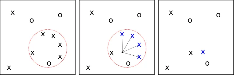
A successful coalescence event.
Simulations
We created a program to simulate, from a Possion-distributed initial configuration (with types drawn from the invariant distribution of the mutation transition matrix). Here, since the environment \(\Pi = (t_i, x_i, r_i, u_i)_{i=1}^\infty\) is independent of the data forward in time, we use a lookdown construction to generate a sample of fixed population size. The animation below shows the simulation run over 2000000 recolonisation and mutation events with the following conditions:
- 30000 lineages on a torus side 30
- Radii law: \( (0.95 \delta_1 + 0.05 \delta_3 )( dr )\)
- Impact law: \( ( \mathbb{ I }_{ \{ 1 \} }( r ) \delta_{ 0.05 } + \mathbb{ I }_{ \{ 3 \} }( r ) \delta_{ 0.3 } )( du ) \)
- Mutation rate: m = 0.05
- Mutation stationary distribution: \( \approx (0.29, 0.30, 0.27, 0.14) \)
Below: Forward-in-time SLFV simulation

We also simulated backwards in time as far at the most recent common ancestor of an initial configuration.
- 10000 lineages on a torus side 10
- Radii law: \( ( 0.95 \delta_1 + 0.05 \delta_3 )( dr ) \)
- Impact law: \( ( \mathbb{ I }_{ \{ 1 \} }( r ) \delta_{ 0.05 } + \mathbb{ I }_{ \{ 3 \} }( r ) \delta_{ 0.3 } )( du ) \)
- Mutation rate: m = 0.05
- Mutation stationary distribution: \( \approx (0.29, 0.30, 0.27, 0.14) \)
Below: Backward-in-time $\Lambda$-coalescent simulation from the proposal distribution outlined in the SMC section