Numerical Results

Table 1: Dimension 1

table1

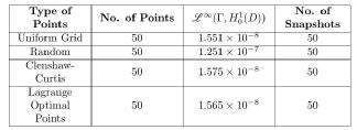
In dimension 1 we choose training sets where the average distance between two neigbouring points is relatively small. This is the reason we get better approximation comparing to higher dimensions. It is clear from Table 1 that the least accurate points are the randomly chosen ones probably because they ignore the fact that there is an underlying structure to the solutions. Thus we expect that the other points have a distribution complimentary to our problem. However, in Table 2 we observe that the Random points perform as well as the other training sets, probably because they become denser.

Table 2: Dimension 1

table1.5.jpeg

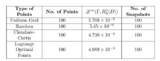
It is difficult to distinguish between different training sets because of the their density in parameter space $\Gamma$ . Thus we now turn our attention to dimension 2.

Table 3: Dimension 2

table2

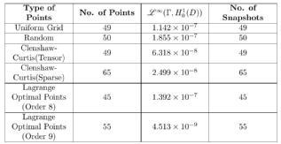
The Uniform grid minimises the maximum distance between any point in $\Gamma$ and a point in our training set. This might lead someone to expect that it would be a good training set. However, it is only as accurate as using the Random
points. This fact suggests that there are some parts of $\Gamma$ which are more important to sample from. Due to the nature of the Lagrange optimal points we are forced to choose a number of the form $\binom{\beta+2}{2}$ (see Table 3). We observe that Order 8 points perform as well as the Random points and the Uniform grid because there are fewer of them compared to the latter points. On the other hand, Order 9 points clearly outperform all the other families despite the fact that there are families with more points. Such a performance can be explained in terms of what was discussed in [3].

Regarding the Clenshaw-Curtis points, in the case of the tensor product we expect such a performance since they are nearly optimal for the minimisation problem (3) and the heuristic explanation above, in terms of what was discussed in [3], applies to this case as well. About the sparse Clenshaw-Curtis, given that they are a good approximation to the full tensor product, one would still expect that they perform well and they do.

Table 4: Dimension 3

table3

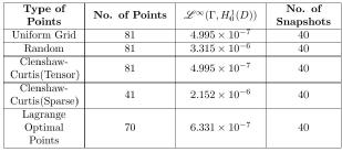
In dimensions 3 and 4 we are beginning to face the curse of dimensionality. For example in dimension 4 if we were to take the tensor product of 1 dimensional training sets, we would have $10^8$ points per training set rather than the approximately 80 that we use. The Lagrange optimal points are quite accurate considering their number and we observe that in dimension 4 the Clenshaw-Curtis sparse grid perform similarly to the Random points even if they are less than half in size. This might be explained again in terms of the reason mentioned in the previous paragraphs.

Table 5: Dimension 4

table4

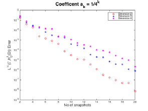
Figures 1,2 and 3

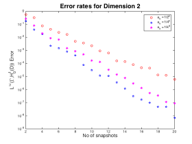
dimension 1 dimension 2 dimension 4

In Figure 1 we notice that the value of the Greedy error is what we expected. The smaller coefficients lead to smaller error. This is basically because the actual coefficient $a(x)=a_0(x)+\sum_{k=1}^K y_k \alpha_k \sin(2\pi kx)$ varies less over $\Gamma$ where $\alpha_k$ are smaller. The decay rates of $\alpha_k=\frac{1}{k^8}$ and $\alpha_k=\frac{1}{4^k}$ are quite similar, while $\alpha_k=\frac{1}{2^k}$ decay at a slower rate.

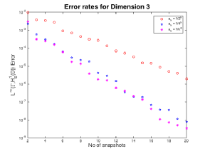
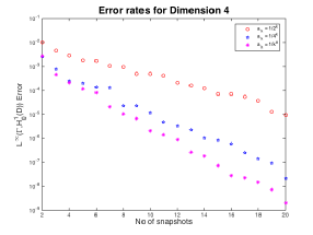
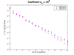
In Figures 2 and 3 we notice that $\alpha_k=\frac{1}{k^8}$ quickly becomes the coefficient with the smallest error as we increase the dimension. This is basically due to the fact that the value of $a(x)$ does not change much as we increase the dimension whereas it does change significantly for the other two coefficients. Furthermore, we see that $\alpha_k=\frac{1}{4^k}$ and $\alpha_k=\frac{1}{k^8}$ have similar decay rates whereas $\alpha_k=\frac{1}{2^k}$ seems to decay with a slower rate, as we previously observed.

At this point we would like to explore the coefficients individually because the behaviour as we increase the dimension seems to be
relevant to what we discussed above.

Figures 4,5 and 6

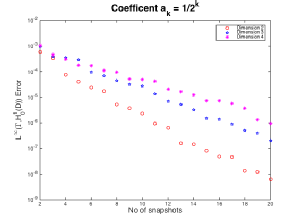
Coefficient 1 coefficient 2 dimension 3

In Figures 4 and 5 we can see that in higher dimensions we have larger error terms, as we expected. In addition as the dimension increases the decay is getting slower, but looks like it's changing less as the dimension is increasing.

In Figure 6 we observe a more interesting behaviour. From results in our report, we expect an algebriac decay of the form $N^{-7}$ . Instead we get an exponential decay which is consistent across all three dimensions, this is probably because with so few dimensions the model cannot "see" that the coefficients have an algebriac decay.

Instead we will look at a slower decay of the coefficients but in higher dimensions specifically sixteen dimensions with $a_k = \frac{1}{k^3}$ .

Figure 7

dimension 16

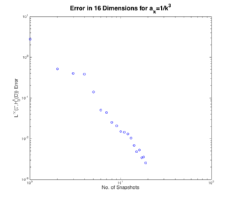
First note that Figure 7 is a log-log scale and so algebraic decay looks linear. The theory form our report indicates that we should expect a decay rate of less than $N^{-2}$ , where in the above figure we got a decay rate of $N^{-2.4}$ .

Figure 8

ErrorEstimator

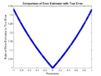
We know that the error estimator is effective (see RBM) in the sense that it bounds the true error and in Figure 8 we can see that this particular error estimator is less than $1.35$ times the true error. Despite this fact the error estimator seems to be systematically worse near the boundary, which implies that the Greedy Algorithm favours points near the boundary.