Sample path large deviations and concentration

Introduction Large Deviation Principles Minimisers of the Rate Function

Introduction

G. Andriopoulos, M. Buze, W. FitzGerald, M. Galton, J. Herman, B. Matharu
Supervisors: S. Adams, R. Tribe

Height functions and law of large numbers

We consider random height fields $\phi=(\phi_i)_{i\in\mathbb{Z}^d}, \phi_i\in\mathbb{R}^m$ over a box $\Lambda_N := \mathbb{Z}^d\cap[0,N]^d$ , distributed under the Gibbs measure

$\gamma_N(\text{d}\phi) := \frac{ e^{-H(\phi)} }{ Z_N } \prod_{i\in\Lambda_N} \text{d}\phi_i$ .

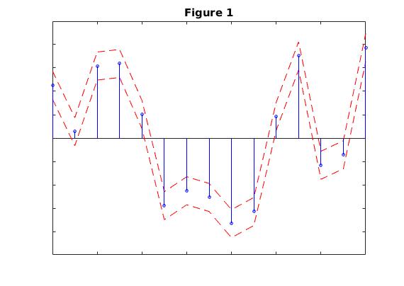
We say these height fields are in $(d+m)-$ dimensions and we may think of this measure returning the probability that a particular height configuration lies within the tube $\text{d}\phi=\left(\text{d}\phi_1,\ldots,\text{d}\phi_N\right)$ . We call the elements of $\phi$ particles, or heights. An example in $(1+1)$ -dimensions is shown in Figure 1. $Z_N$ is a normalising factor, called the partition function , and ensures our measure is a probability measure. $H$ is the Hamiltonian for our system, and takes the form $H(\phi) = \sum_{i\in\Lambda_N}V(\Delta\phi_i)$ , where $\Delta\phi_i=\phi_{i+1}-2\phi_i+\phi_{i-1}$ is the discrete Laplacian and $V$ is called the Potential, discussed later. In our case, the boundary is given by $\partial\Lambda_N= \{-1,0,\ldots,N,N+1\}$ .

Note: The boundary $\partial\Lambda_N$ and microscopic height functions $h^N$ differ when $V(\eta)$ differs, depending on $\eta$ . This is called the Particle Interaction and is discussed under a later sub-heading.

To impose boundary conditions $\psi$ on our height field $\phi$ , we adapt our measure to take the form

$\gamma_N^{\psi}(\text{d} \phi) := \frac{ e^{-H(\phi)} }{ Z_N^\psi }\prod_{i\in\Lambda_N}\text{d}\phi_i\prod_{ i\in\partial\Lambda_N }\delta_{\psi_i}(\text{d}\phi_i)$

We can see the extra product at the end of the right hand side will ensure our boundary conditions are satisfied, else we see the probability of finding a height configuration without the boundary conditions $\psi$ to be zero.
From these height fields, we can define the macroscopic height functions as follows:

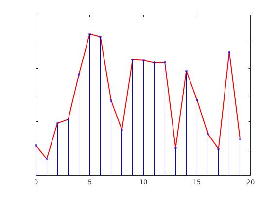
$N^2 h^N(t) =\phi_{ \lfloor Nt\rfloor } + \left(t - \frac{\lfloor Nt\rfloor}{N} \right)( \phi_{\lfloor Nt\rfloor + 1} - \phi_{\lfloor Nt\rfloor} )$

Below we can see some typical height fields for various $N$ , pictured in blue, and their corresponding height functions (before scaling) in red. Notice that as $N\rightarrow \infty$ , our height functions appear to be converging.

Our overall aim is to find a Law of Large numbers for $h^N, (N\rightarrow\infty)$ .

Finding LLNs for $h^N$ is acheived through the use of large deviations. Indeed, minimisers of the rate function associated to the measures $(\gamma_N^\psi)_{N\in\mathbb{N}$ correspond to LLNs for the height functions $h^N$ for a suitable class of admissable functions. For instance, in $(1+ 1)$ -dimensions we take the space $H^2_{\bm{a,b} }([0,1]) := \left\{h\in H^2([0,1]) : h(0)=a,h(1)=b,h'(0)=\alpha,h'(1)=\beta\right\}$ for the problem with both end points and initial velocities fixed.

By changing our measure $\gamma_N^\psi$ , we may consider different variants of the model we have introduced here. For example, we may force our particles to be positive (wetting), or even give our particles an attraction the the '0 line' (pinning). These cases are discussed under later sub-headings.

Potentials

The potential $V$ always undergoes the assumptions

$\int_\mathbb{R} \operatorname{exp}(-V(x)) \text{d}x \text{\textless} \infty$
$\int_\mathbb{R} x\operatorname{exp}(-V(x)) \text{d}x = 0$
$\int_\mathbb{R} x^2\operatorname{exp}(-V(x)) \text{d}x \text{\textless} \infty$

Occasionally, we make the stronger assumptions

$V$ is twice continuously differentiable.
$V$ is symmetric, $V(x)=-V(x)$
$V$ is strictly convex, $\exists c_1,c_2:c_1\leq V''(x)\leq c_2$ .

The potential usually considered is the Gaussian potential, $V(\eta)=\frac{1}{2}\eta^2$ . This has many advantages as Gaussian potentials yield very nice bounds, due to Gaussian calculus.
The other potential often considered is of general type, needing only satisfying the assumptions above.

Particle Interactions

There are two types of particle interactions that are commonly considered, one is called the Gradient interaction, and the other is the Laplacian interaction.

The laplacian case is defined by the interactions $V( \Delta\phi_i) = V(\phi_{i+1} - 2 \phi_i + \phi_{i-1}), i=1,\ldots,N-1$ . For this, we take our boundary to be $\partial\Lambda = \{ -1,0,N,N+1\}$ .

Note: We will consider the laplacian interaction throughout.

The gradient case is defined by the interaction $V(\eta) = V(\phi_i - \phi_{i-1}), \ i = 1,\ldots, N$ . Here we take a boundary of the form $\partial \Lambda = \{ 0, N \}$ . Unlike the Laplacian interaction, the height functions undergo a scaling by a factor $N$ , so we consider $N h^N(t)$ , instead of considering $N^2 h^N(t)$ . The majority of the work in this area has been dedicated to the gradient case, and as such there are many results for this type of particle interaction. This case is easier than the Laplacian case, as potentials considered with a gradient interaction have the markov property, and hence may be considered as random walks. This gives us extra theory to get bounds for large deviations.

Pinning

Pinning can be loosely be described as 'an attraction to the 0 line'. More precisely, it is defined as a limit of a particular choice of potentials. In the limit, we obtain Pinning through the measure

$\gamma_N^{\psi,\epsilon}(\text{d} \phi) := \frac{ e^{-H(\phi)} }{ Z_N^\psi }\prod_{i\in\Lambda_N}\left(\text{d}\phi_i+\epsilon\delta_0(\text{d}\phi_i)\right)\prod_{ i\in\partial\Lambda_N }\delta_{\psi_i}(\text{d}\phi_i).$

As we can see, the extra term $\delta_0(\text{d}\phi)$ corresponds giving our height fields $\phi$ a 'reward' for touching the '0 line'.

Wetting

Wetting is when we force our height functions to be positive everywhere. Unlike the case of pinning, wetting is conditioned on to our measure in a hard fashion by considering $\gamma( \cdot | \phi \geq 0 )$ . In the case of wetting, our analysis becomes more interesting as we minimise over the convex space $K := \left\{ h \in H^2_{\bm{a,b} } : h \geq 0 \right\}$ , which gives rise to obstacle and free boundary problems.

Acknowledgements

We acknowledge the funding body EPSRC and the support from MASDOC CDT.

MASDOC logo EPSRC logo