Sample path large deviations and concentration

Introduction Large Deviation Principles Minimisers of the Rate Function

Large Deviation Principles

This LDP is for a Laplacian particle interaction, Gaussian potential with Wetting.

We take our measure to be of the form

$\gamma_{N}^{\bm{a,b},+}(\text{d}\phi) := \frac{ e^{-H(\phi)} }{ Z_N } \prod_{i=1}^{N-1} \text{d}\phi_i 1(\phi_i \geq 0)$

with boundary conditions $\bm{a,b}$ imposed at $\phi_{-1}, \phi_0, \phi_N, \phi_{N+1}$ .
Define the space

$K_\bm{a,b} := \{ h\in C([0,1]):h\geq0, h(0)=a,h'(0)=\alpha, h(1) = b, h'(1) = \beta \}$

and the rate function

$I^+(h):= \begin{cases} \Sigma^\Delta(h) - \inf_{g\inX}\Sigma^\Delta(g), & h\in X \\ \infty, & h\notin X \end{cases}$

where $X=K_\bm{a,b}$ and

$\Sigma^\Delta(h):= \frac{1}{2} \int_0^1 (h''(t))^2 \text{d}t.$

We then obtain the following:

Theorem: The empirical profiles $h_N$ under the measures $\left(\gamma_{N}^{\bm{a,b},+}\right)_{N}$ satisfy an LDP on the space $K_\bm{a,b}$ with rate $N$ and rate function $I^+(h)$ .

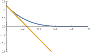
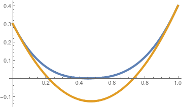
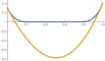
Note that this theorem is for the Dirichlet boundary, with Gaussian potential. The wetting in this theorem imposes difficulties as our minimisers will have to change if there is a large initial downward gradient with a starting point near the origin. A few examples of how wetting changes minimisers is shown below. The orange lines represent a typical minimiser without wetting, and its corresponding minimiser with wetting is shown in blue.

The proof of this theorem involves a technical lemma which we state without proof

Lemma: There exists a coupling of random variables constructed on a common probability space such that $|h^\bm{(a,b)}_N - h^{\bm{(a,b)}+z}_N|\leq|z|$ where $h^\bm{(a,b)+z}_N$ is the macroscopic height variable distributed according to the measure $\gamma_{N,\bm{(a,b)}+z}^+$ , with boundary $\bm{a}$ .

The main difficulty in the proof of the theorem is when the boundary values are zero. This introduces a technical problem that open sets in the space of continuous fuctions consistent with these boundary values contan functions which take negative values. The key lemma is used in the proof to 'lift' our boundary values away from zero and overcome this difficulty.

Note: This Theorem has also been shown in the free boundary case, with general potential V.