Kalman Filtering

Kalman filtering is an algorithm that tries to reconcile outputs from a mathematical model of a physical system and observations of the same system. It combines these two in such a way as to smooth out noise coming from inaccurate observations in an effort to more accurately estimate the true state of the system at the present time.

Consider the process $x\in \mathbb{R}^d$ given by the stochastic difference equation
$x^i=Ax^{i-1}+Bu^{i-1}+w^{i-1}$
with $u$ the control variables, and consider also measurements
$z^i = Hx^i +v^i$
where $w$ and $v$ represent noise terms, and are assumed to be independent multivariate normals with distributions
$w \sim \text{MVN}(0,Q) \hspace{2cm} v\sim \text{MVN}(0,R).$
It should be recognised that this is somewhat of a special case of the usual Kalman filter, because one may well expect the noise to vary over time, and so then the above would be indexed by $i$ .

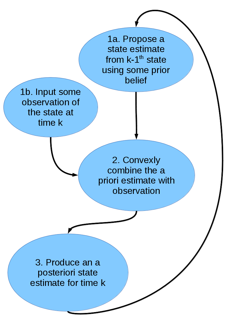
The algorithm is as follows

At time $n$ , given the previous a posteriori estimates $x^{n-1},...,x^{n-l}$ of the system, a prediction $\widehat{x}^{n|n-1}$ is made based upon the prior belief or physical dynamics of the system at time $n$ .
The system is observed at time $n$ and this observation $z^{n}$ is used to correct the a priori estimate $\widehat{x}^{n|n-1}$ and produce an updated estimate $\widehat{x}^{n|n}$ .
Repeat for time $n+1$ .

The above algorithm handles the case that the update as linear. There is absolutely no reason to expect this to be the case and the algorithm can be altered to allow for non-linearities. In the non-linear case we must add a step in the procedure so that we can make the linear Kalman filter applicable. This new procedure is called the extended Kalman filter.
Here, instead of having a relation as in the first equation we have a relation
$x^{i+1} = f(x^{i},u^i) +w^i$
where $f$ is non-linear, and $w$ is again the noise term, and we have measurements
$z^i = h(x^i)+v^i.$
Now we assume, if $f,h \in C^1$ , with derivatives $F$ and $H$ respectively, that the estimate is given by
$\widehat{x}^{i+1}\sim \mathcal{N}(Df(m^i), Df(m^i)^TC^i Df(m^i))$
for some $m^i$ and $C^i$ to be determined and we have
$\widehat{x}^{i+1|i} \sim N (\widehat{x}^{i+1|i} + K(y^i - h(\widehat{x}^{i+1|i})))$
where K is the so-called Kalman gain matrix. Observe that this linearises the problem, and we thus use the linear Kalman filter as above on this model. This however may be poor if our function $f$ is highly non-linear.

The main advantage of using the Kalman filter in practice is that it finds solutions to an estimation problem sequentially and thus reduces the computational cost and time so that it can be performed as and when an observation is made.