
1D stochastic Allen-Cahn with asymmetric potential
Before reading this section it may be helpful to see some motivation and animations.
Recall that the 1D-SACE equation is given by
$(1)\hspace{0.5cm}\displaystyle\frac{\partial u}{\partial t} = \frac{1}{2}\frac{\partial^2 x }{\partial x^2} + f_{\varepsilon}(u) + \sigma \varepsilon^{1/2} \xi$
and that we consider an asymmetric potential so that $f_{\varepsilon} = u - u^3 - c\varepsilon (1-u^2)$.
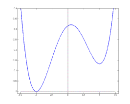
You can see at the right the asymmetric potential that we consider with $c\varepsilon = 0.1$. Please note
that it still has (local) minima at $\pm 1$.
The concept of instantons and centres play a key role in our analysis. Before reading further, make sure that you understand these concepts.
Main result
The centre of any solution to the 1D-SACE (1) with asymmetric potential for which $f_{\varepsilon}(u)=u-u^3-c\varepsilon(1-u^2)$ and initial condition close to an instanton moves, as $\varepsilon\rightarrow 0$, as a Brownian motion with drift parameter $c$.
We introduce a moving coordinate system transformation $(x,t) \rightarrow (y,t)$ where $y = x -c\varepsilon t$, which results in a moving frame. Using the chain rule, we obtain the following equation in the moving frame:
$\displaystyle\frac{\partial u}{\partial t} = \frac{1}{2}\frac{\partial^2 u }{\partial y^2} +c\varepsilon \frac{\partial u}{\partial y} + \left[ u-u^3 \right] - c\varepsilon\left[ 1-u^2 \right] + \varepsilon^{1/2} \xi = 0$.
Sketch proof:
We call $p$ the solution to the 1D-SACE in the moving frame and then we:
- Prove that $p$ satisfies similar properties to the solution in the non-moving frame: bounded by 2 and weak comparison principle.
- Show that $p$ is close to an instanton whose centre moves, in the moving frame, as a Brownian motion with no drift.
- Conclude that the centre of the solution of the 1D-SACE in the non-moving frame moves like a Brownian motion with drift determined by the speed of the moving frame.
To check our numerical results on the 2D-SACE please click here.