Now, with possible values for our parameters, the basic idea is to simulate our model and see if we are able to recover our original data.

First, we simulate our three parameter model. The results are shown in the next graph:

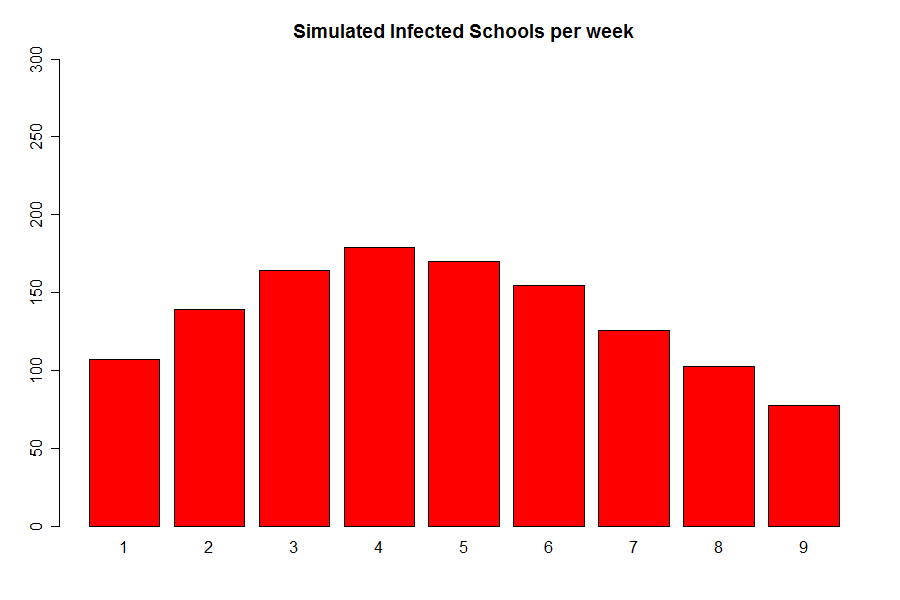
Since, its peak is considerably below the actual epidemic we decided to include the extra parameter and to increment the amount of infected schools:

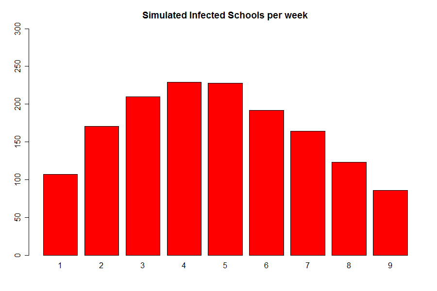
• The parameter will detect external pressure to the schools, increasing the value of as already explained on the model section. This will increase the amount of schools infected at each week.
• The parameter will control the shape of the infectious period of school , , which originally was considered as a Geometric() random variable, that is the discrete equivalent to the exponential distribution. Now, it is a Negative Binomial (, ), that is the discrete equivalent to the Gamma distribution. The main idea of this, is to reduce the probability assigned to lower values of and increase the probability of higher values. In that way, schools are more likely to stay infected for a longer period.

Now, consider this 5 parameter model, we obtain the following graph:

Finally, we were also available to illusrate the evolution of this simulated epidemic through time:

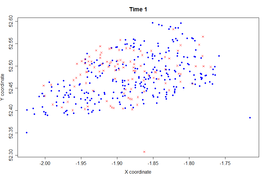
Key:

Blue - Susceptible

Red - Infected

Green - Recovered

For quantitative results one could look at:

Simulation Results

Public Policy