Manual for previous SnPM versions
|
|
PET example |
This page... introduction example data background design setup computation viewing results SnPM pages... manual PET example fMRI example FSL users |
SnPM exampleIn this section we analyze a simple motor activation experiment with the SnPM software. The aim of this example is three-fold:
|
The Example Data
This example will use data from a simple primary motor activation experiment. The motor stimulus was the simple finger opposition task. For the activation state subjects were instructed to touch their thumb to their index finger, then to their middle finger, to their ring finger, to their pinky, then repeat; they were to do this at a rate of 2 Hz, as guided by a visual cue. For baseline, there was no finger movement, but the visual cue was still present. There was no randomization and the task labeling used was
- A B A B A B A B A B A B
You can down load the data from ftp://www.fil.ion.ucl.ac.uk/spm/data/PET_motor.tar.gz or, in North America, from ftp://rowdy.pet.upmc.edu/pub/outgoing/PET_motor.tar.gz. We are indebted to Paul Kinahan and Doug Noll for sharing this data. See this reference for details: Noll D, Kinahan et al. (1996) "Comparison of activation response using functional PET and MRI" NeuroImage 3(3):S34.
Currently this data is normalized with SPM94/95 templates, so the activation site will not map correctly to ICBM reference images.
Before you touch the computer
The most important consideration when starting an analysis is the choice of exchangeability block size and the impact of that choice on the number of possible permutations. We don't assume that the reader is familiar with either exchangeability or permutation tests, so we'll attempt to motivate the permutation test through exchangeability, then address these central considerations.
Exchangeability
First we need some definitions.
- Labels & Labelings A designed experiment entails repeatedly collecting data under conditions that are as similar as possible except for changes in an experimental variable. We use the term labels to refer to individual values of the experimental variable, and labeling to refer to a particular assignment of these values to the data. In a randomized experiment the labeling used in the experiment comes from a random permutation of the labels; in a non-randomized experiment the labeling is manually chosen by the experimenter.
- Null Hypothesis The bulk of statistical inference is built upon what happens when the experimental variable has no effect. The formal statement of the "no effect" condition is the null hypothesis.
- Statistic We will need to use the term statistic in it's most general sense: A statistic is a function of observed data and a labeling, usually serving to summarize or describe some attribute of the data. Sample mean difference (for discrete labels) and the sample correlation (for continuous labels) are two examples of statistics.
We can now make a concise statement of exchangeability. Observations are said to be exchangeable if their labels can be permuted with out changing the expected value of any statistic. We will always consider the exchangeability of observations under the null hypothesis.
We'll make this concrete by defining these terms with our data, considering just one voxel (i.e 12 values). Our labels are 6 A's and 6 B's. A reasonable null hypothesis is ``The A observations have the same distribution as the B observations''. For a simple statistic we'll use the difference between the sample means of the A & B observations. If we say that all 12 scans are exchangeable under the null hypothesis we are asserting that for any permutation of A's and B's applied to the data the expected value of the difference between A's & B's would be zero.
This should seem reasonable: If there is no experimental effect the labels A and B are arbitrary, and we should be able to shuffle them with out changing the expected outcome of a statistic.
But now consider a confound. The most ubiquitous confound is time. Our example data took over two hours to collect, hence it is reasonable to suspect that the subject's mental state changed over that time. In particular we would have reason to think that difference between the sample means of the A's and B's for the labeling
- A A A A A A B B B B B B
would not be zero under the null because this labeling will be sensitive to early versus late effects. We have just argued, then, that in the presence of temporal confound all 12 scans are not exchangeable.
Exchangeability Blocks
The permutation approach requires exchangeability under the null hypothesis. If all scans are not exchangeable we are not defeated, rather we can define exchangeability blocks (EBs), groups of scans which can be regarded as exchangeable, then only permute within EB.
We've made a case for the non-exchangeability of all 12 scans, but what if we considered groups of 4 scans. While the temporal confound may not be eliminated its magnitude within the 4 scans will be smaller simply because less time elapses during those 4 scans. Hence if we only permute labels within blocks of 4 scans we can protect ourselves from temporal confounds. In fact, the most temporally confounded labeling possible with an EB size of 4 is
- A A B B A A B B A A B B
Number of Permutations
This brings us to the impact of EB size on the number of permutations. The table below shows how EB size affects the number of permutations for our 12 scan, 2 condition activation study. As the EB size gets smaller we have few possible permutations.
| EB size | Num EB's | Num Permutations | ||
| 12 | 1 | 12C6 | = | 924 |
| 6 | 2 | (6C3)2 | = | 400 |
| 4 | 3 | (4C2)3 | = | 216 |
| 2 | 6 | (2C1)6 | = | 64 |
This is important because the crux of the permutation approach is calculating a statistic for lots of labelings, creating a permutation distribution. The permutation distribution is used to calculate significance: the p-value of the experiment is the proportion of permutations with statistic values greater than or equal to that of the correct labeling. But if there are only, say, 20 possible relabelings and the most significant result possible will be 1/20=0.05 (which would occurs if the correctly labeled data yielded the largest statistic).
Hence we have to make a trade off. We want small EBs to ensure exchangeability within block, but very small EBs yield insufficient numbers of permutations to describe the permutation distribution well, and hence assign significance finely. We usually will use the smallest EB that allows for at least hundreds of permutations (unless, of course, we were untroubled by temporal effects).
Design Setup
It is intended that you are actually sitting at a computer and are going through these steps with Matlab. We assume that you either have the sample data on hand or a similar, single subject 2 condition with replications data set.
First, if you have a choice, choose a machine with lots of memory. We found that this example causes the Matlab process to grow to at least 90MB.
Create a new directory where the results from this analysis will go. Either start Matlab in this directory, or cd to this directory in an existing Matlab session.
Start SnPM by typing
- snpm
which will bring up the SnPM control panel (and the three SPM windows if you haven't started SPM already). Click on
- Setup
A popup menu will appear. Select the appropriate design type from the the menu. Our data conforms to
- Single Subject: 2 Conditions, replications
It then asks for
- # replications per conditions
We have 6.
Now we come to
- Size of exchangeability block
From the discussion above we know we don't want a 12-scan EB, so will use a EB size of 4, since this gives over 200 permutations yet is a small enough EB size to protect against severe temporal confounds.
- The help text for each SnPM plug in file gives a formula to calculate the number of possible permutations given the design of your data. Use the formula when deciding what size EB you should use.
It will now prompt you to select the image data files. In the prompted dialog box, you need to input the correct file directory, and then click on the image data files (.img) one by one. It is important that you enter them in time order. Or you can click on All button if you want to choose all the files. After you finish choosing all of the files, click on "Done".
Next you need to enter the ``conditions index.'' This is a sequence of A's and B's (A's for activation, B's for baseline) that describe the labeling used in the experiment. Since this experiment was not randomized we have a nice neat arrangement:
- A B A B A B A B A B A B
Exchangeability Business
Next you are asked about variance smoothing. If there are fewer than 20 degrees of freedom available to estimate the variance, variance smoothing is a good idea. If you have around 20 degrees of freedom you might look at at the variance from a SPM run (Soon we'll give a way to look at the variance images from any SPM run). This data has 12-2-1=9 degrees of freedom at each voxel, so we definately want to smooth the variance.
It is our experience that the size of the variance smoothing is not critical, so we suggest 10 mm FWHM variance smoothing. Values smaller than 4 mm won't do much smoothing and smoothing probably won't buy you anything and will take more time. Specify 0 for no smoothing.
The next question is "Collect Supra-Threshold stats?" The default statistic is the maximum intensity of the t-statistic image, or max pseudo-t if variance smoothing is used. If you would like to use the maximum supra-threshold cluster size statistic you have to collect extra data at the time of the analysis. Beware, this can take up a tremendous amount of disk space; the more permutations the more disk space required. This example generates a 70MB suprathreshold statistics mat file. Answer 'yes' to collect these stats. Or click on 'no' to save some disk space.
The remaining questions are the standard SPM questions. You can choose global normalization (we choose 3, Ancova), choose 'global calculation' (we choose 2, mean voxel value), then choose 'Threshold masking' (we choose proportion), and keep 'Prop'nal threshod' as its default 0.8. Choose 'grand mean scaling' (we choose 1, scaling of overall grand mean) and keep 'scale overall grand mean' at its default 50. the gray matter threshold (we choose the default, 0.8) and the value for grand mean (again we choose the default, 50).
Now SnPM will run a short while while it builds a configuration file that will completely specify the analysis. When finished it will display a page (or pages) with file names and design information. When it is finished you are ready to run the SnPM engine.
Computing the nonParametric permutation distributions
In the SnPM window click on
- Compute
You will be asked to find the configuration file SnPM has just created (It should be in the directory where you run matlab); it's called
- SnPM_cfg.mat
Some text messages will be displayed and the thermometer progress bar will also indicate progress.
On fast new machines, like Sun Sparc Ultras or a Hewlett Packard C180, the computation of permutation should only take about 5 minutes.
One of the reasons that SnPM is divided into 3 discrete operations (Configure, Compute, Results) is to allow the Compute operation to be run at a later time or in the background. To this end, the 'Compute' function does not need any the windows of SPM and can be run with out initializing SPM (though the MATLABPATH environment variable must be set). This maybe useful to remember if you have trouble with running out of memory
To maximize the memory available for the 'Compute' step, and to see how to run it in batch mode, follow these steps.
- If running, quit matlab
- In the directory with the SnPM_cfg.mat file, start matlab
- At the matlab prompt type
- snpm_cp .
This will 'Compute' just as before but there will be no progress bar. When it is finished you could type 'spm PET' to start SPM99, but since Matlab is not known for it's brilliant memory management it is best to quit, then restart matlab and SnPM.
On a Sun UltraSPARC 167 MHz this took under 6 minutes.
Results
In the SnPM window click on
- Results
You will be asked to find the configuration file SnPM has just created; it's called
- SnPM.mat
Next it will prompt for positive or negative effects. Positive corresponds to ``A-B'' and negative to ``B-A''. If you are interested in a two tailed test repeat this whole procedure twice but halve your p value threshold value in the next entry.
Then, you will be asked questions such as 'Write filtered statistic img?' and 'Write FWE-corrected p-value img?'. You can choose 'no' for both of them. It will save time and won't change the final result.
Next it will ask for a corrected p value for filtering. The uncorrected and FWE-corrected p-values are exact, meaning if the null hypothesis is true exactly 5% of the time you'll find a P-value 0.05 or smaller (assuming 0.05 is a possible nonparameteric P-value, as the permutaiton distribution is discrete and all p-values are multiples of 1/nPerm). FDR p-values are valid based on an assumption of positive dependence between voxels; this seems to be a reasonable assumption for image data. Note that SPM's corrected p values derived from the Gaussian random field theory are only approximate.
Next, if you collected supra-threshold stats, it will ask if you want to assess spatial extent. For now, let's not assess spatial extent.
You will be given the opportunity to write out the statistic image and the p-value image. Examining the location of activation on an atlas image or coregistered anatomical data is one of the best way to understand your data.
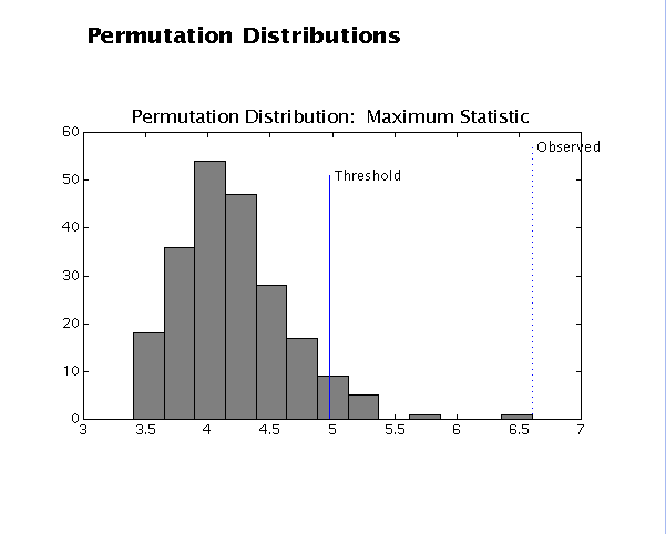
Shortly the Results screen will first show the permutation distributions.

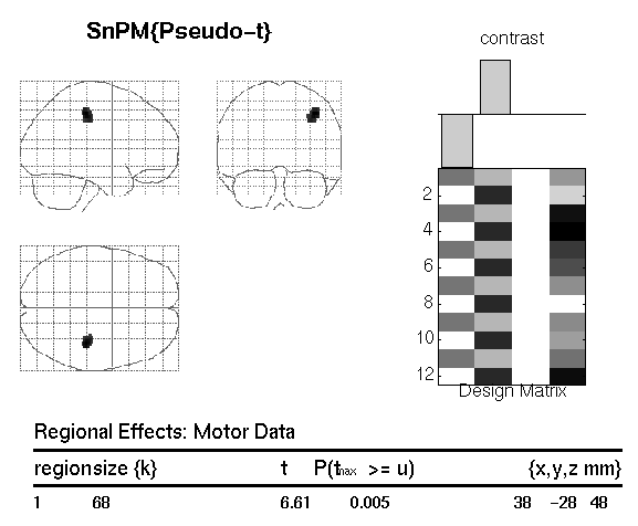
You need to hit the ENTER button in the matlab main window to get the second page. The screen will show the a maximum intensity projection (MIP) image, the design matrix, and a summary of the significantly activated areas.

The figure is titled ``SnPM{Pseudo-t}'' to remind you that the variance has been smoothed and hence the intensity values listed don't follow a t distribution. The tabular listing indicates that there are 68 voxels significant at the 0.05 level; the maximum pseudo-t is 6.61 and it occurs at (38, -28, 48).

This information at the bottom of the page documents the parameters of the analysis. The ``bhPerms=1'' is noting that only half of the permutations were calculated; this is because this simple A-B paradigm gives you two labelings for every calculation. For example, the maximum pseudo-t of the
-
A A B B B B A A A A B B
labeling is the minimum pseudo-t of the
-
B B A A A A B B B B A A
labeling.
Now click again on
Results
proceeding as before but now answer Yes when it asks to assess spatial extent. Now you have to decide on a threshold. This is a perplexing issue which we don't have good suggestions for right now. Since we are working with the pseudo-t, we can't relate a threshold to a p-value, or we would suggest a threshold corresponding to, say, 0.01.
When SnPM saves supra-threshold stats, it saves all pseudo-t values above a given threshold for all permutations. The lower lower limit shown (it is 1.23 for the motor data) is this ``data collection'' threshold. The upper threshold is the pseudo-t value that corresponds to the corrected p-value threshold (4.98 for our data); there is no sense entering threshold above this value since any voxels above it are already significant by intensity alone.
Trying a couple different thresholds, we found 2.5 to be a good threshold. This, though, is a problem. The inference is strictly only valid when the threshold is specified a priori. If this were a parametric t image (i.e. we had not smoothed the variance) we could specify a univariate p-value which would translate to specify a t threshold; since we are using a pseudo t, we have no parametric distributional results with which to convert a p-value into a pseudo t. The only strictly valid approach is to determine a threshold from one dataset (by fishing with as many thresholds as desired) and then applying that threshold to a different dataset. We are working to come up with guidelines which will assist in the threshold selection process.

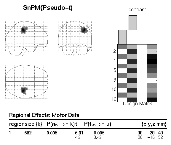
Now we see that we have identified one 562 voxel cluster as being significant at 0.005 (all significances must be multiples of 1 over the number of permutations, so this significance is really 1/216=0.0046). This means that when pseudo-t images from all the permutations were thresholded at 2.5, no permutation had a maximum cluster size greater than 562.
-
Back to main SnPM page
-
SnPM by Andrew Holmes of the Astra Zeneca
& Tom Nichols of University of Michigan Biostatistics department
-
SnPMauthors at <snpm-authors at umich.edu>
Neuroimaging
Statistics
Contact Info
Room D0.03
Deptment of Statistics
University of Warwick
Coventry
CV4 7AL
United Kingdom
Tel: +44(0)24 761 51086
Email: t.e.nichols 'at' warwick.ac.uk
Web: http://nisox.org
Blog: NISOx blog
Handbook of fMRI Data Analysis by Russ Poldrack, Thomas Nichols and Jeanette Mumford


![[Book Cover]](https://warwick.ac.uk/fac/sci/statistics/staff/academic-research/nichols/publications/books/handbookfmri_cover.jpg?maxWidth=125)