Detecting Blebs

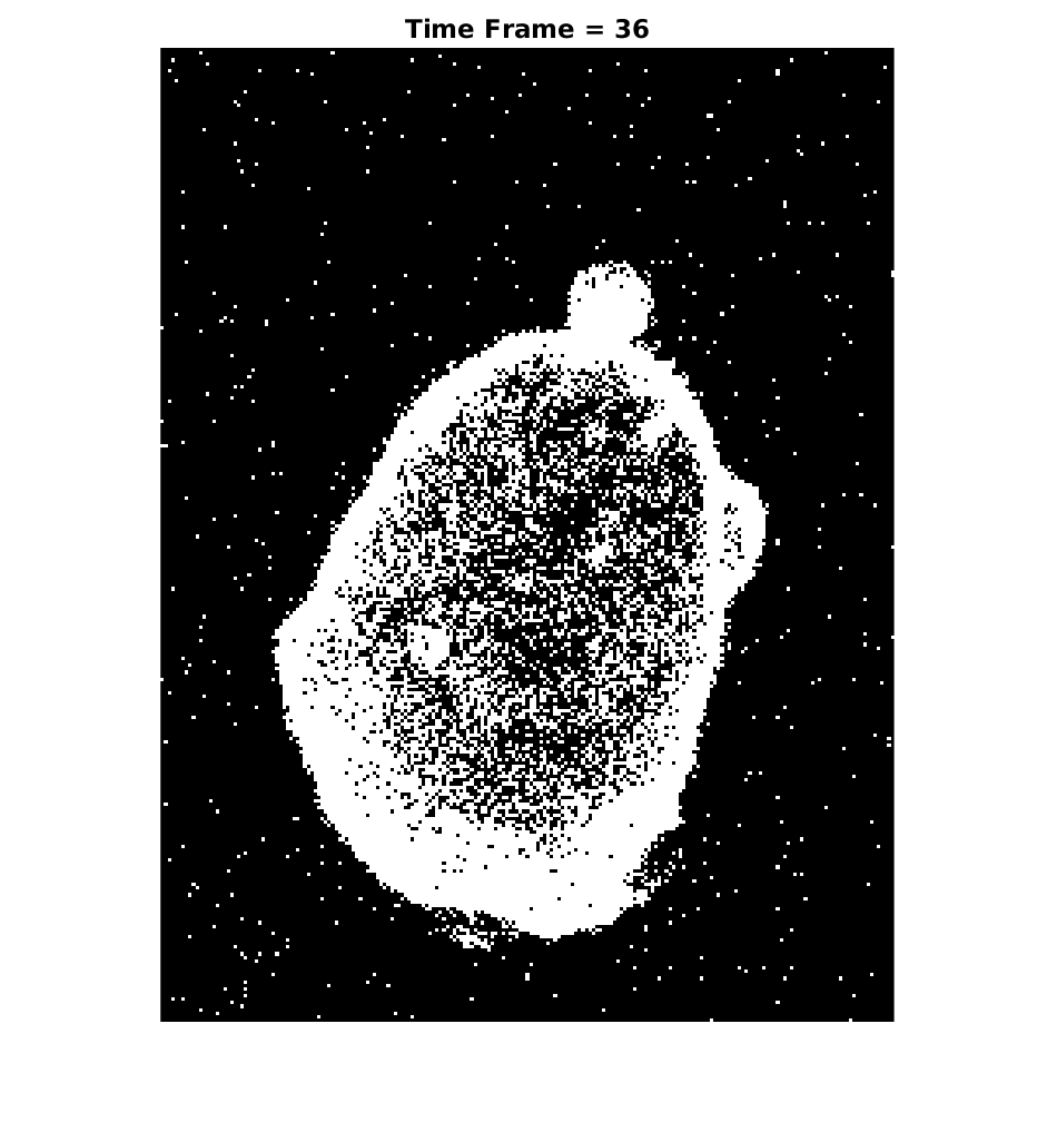
We start with a given sequence of grayscale images representing the time series of the blebbing cell. These images are interpreted in MatLab as matrices with entries between 0 and 255. These matrices are then converted into binary by setting entries that correspond to pixels of intensity less than than some threshold to zero. Now, we look at the difference of the matrices representing consecutive frames of the cell and set negative values in this difference matrix to zero. Non-zero entries of the difference matrix therefore represent the change in the cell from one time frame to the next. We shall assume that blebs are connected clusters of pixels, which means that we are interested in detecting whether or not connected components of the difference matrices are in fact blebs. The animated gif (right) illustrates the above described procedure.

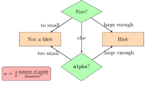In order to decide whether or not each connected component is a bleb, we look at the size and "roundness" of each connected component. Here the size refers to the number of non-zero pixels in the connected component and the roundness is calculated using the formula

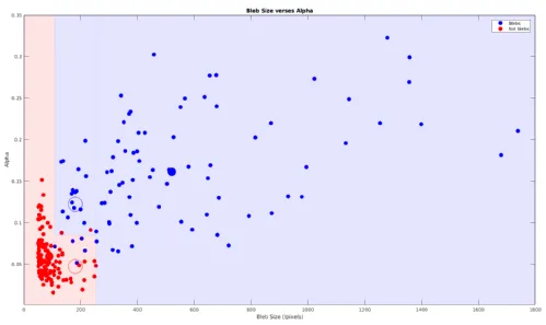
We then use the decision tree (right) to determine whether or not each connected component is a bleb. Here, "large enough" and "too small" refer to the quantity being larger than or smaller than lower and upper bleb size thresholds and a roundness threshold . We viewed finding these thresholds as a machine learning problem where we use the given data (the images) in order to come up with a suitable definition of a bleb that accurately reflects the underlying biological setting. The plot (right) shows the actual blebs (in blue) as well as the connected components of the difference matrix that are not blebs (in red) together with the thresholds we found.

Assigning Blebbing Intensities

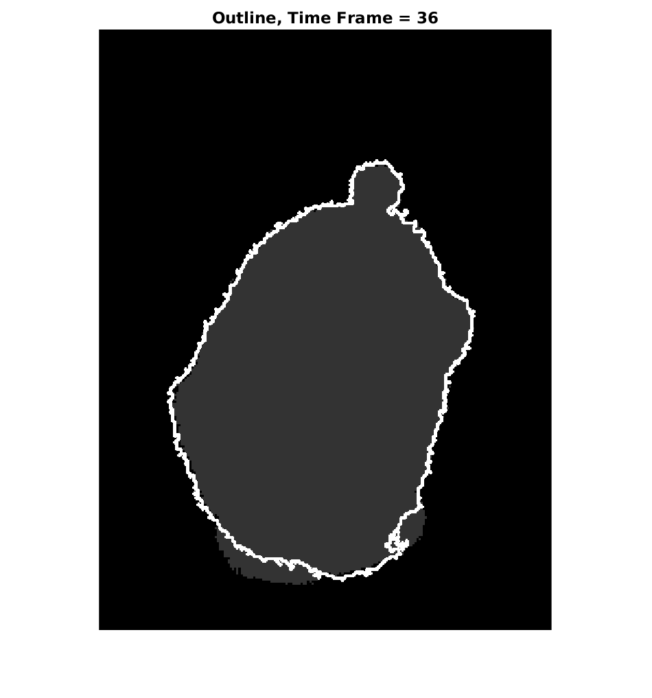
Now we come to assigning blebbing intensities to the inside edge of the bleb. Firstly, we use standard MatLab functions to get the outside boundary of the cell. We are interested in assigning non-zero intensities to that part of the boundary that blebbed and zero intensities elsewhere. We now look at all the pixels that are both on the boundary of the cell and part of the bleb. This gives us the inside edge of the bleb. We wish to assign the values 3, 2 and 1 to the bleb edge moving from the centre of the bleb towards the endpoints. In order to do this we first estimate the centre of the cell and use this to measure the angle between points of the bleb edge. Maximising the angle between two points of the bleb edge gives us the two endpoints. Now for each pixel on the bleb edge we calculate the angle between the pixel and one of the bleb endpoints. Depending on this angle, we assign the blebbing intensities. In the animated gif (right), red points on the bleb edge correspond to intensity 3, yellow points have intensity 2 and green have intensity 1.

Links:

Homepage

HMM

Prototype Model

Image Analysis

Code

---

H. Bharth
J. Kiedrowski
J. Sant
J. Thomas

Supervised by:
Dr Björn Stinner
Dr Stefan Adams