WEEK 1-2

These weeks were a training period to be able to complete some of the necessary techniques and analysis independently.

The techniques that I learnt in the first week were infiltration; DNA extraction; running gels and using cameras to take images of the infiltrated plants to check the progression of the disease. Each procedure presented its unique challenges.

Infiltration was the most difficult as my job was to prepare bacteria solution and inject it into the leaf after wounding, it is very easy to damage your plants. For example, to make the infiltration easier I always try not to leave too much time between wounding and infiltration!
This would require you to cut the leaf again as the original cut healed, inflicting further stress. Another aspect not to forget is to dispose the waste into the correct autoclaved waste disposal sites since we are using licensed bacteria. This technique will take a lot of practice before I can move on the lines provided by Laura.

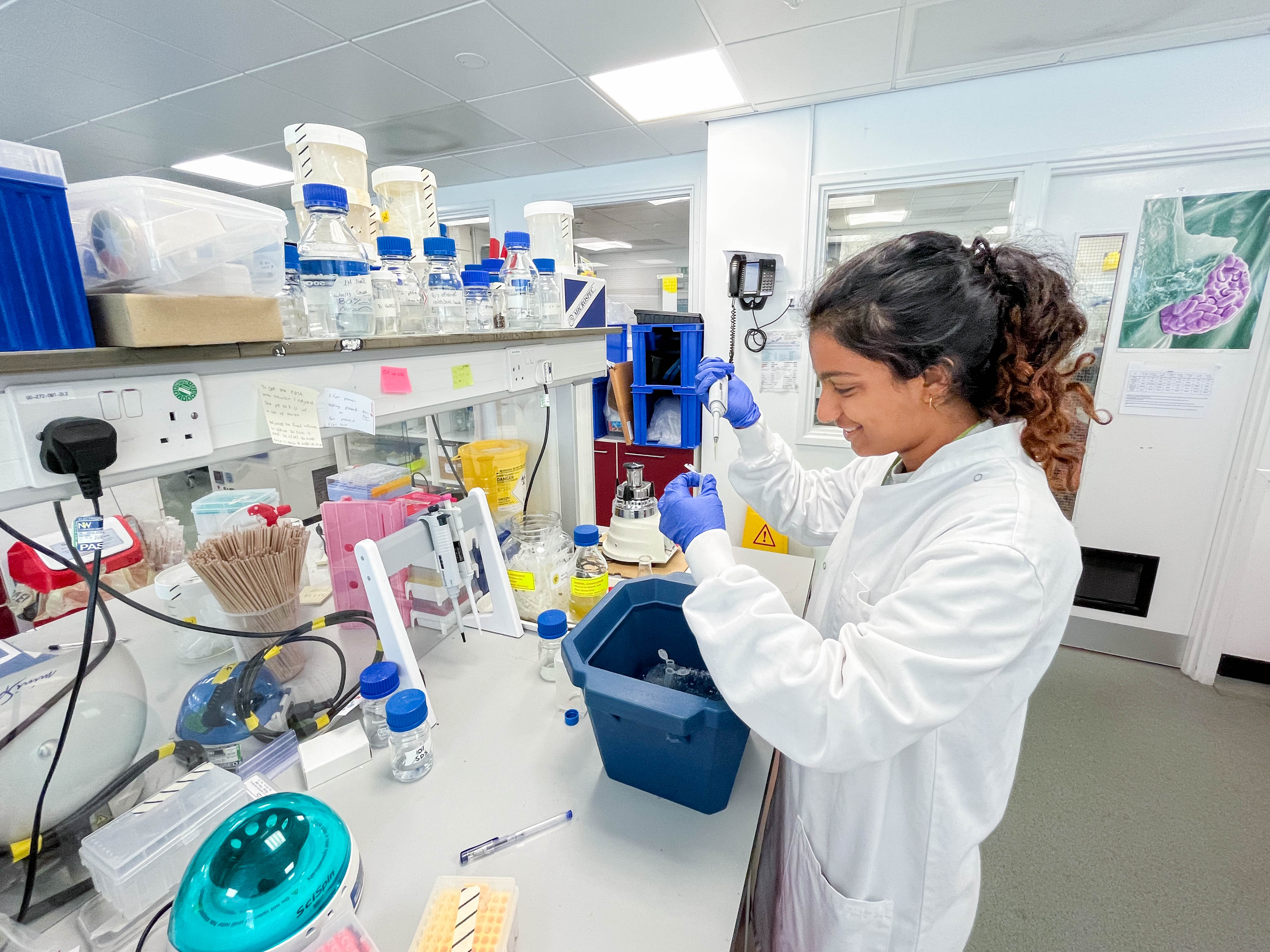
Performing a DNA extraction requires making a buffer solution that can easily precipitate if left too long on its own. This means finding ways to optimise time is crucial to maximise the quality of the DNA extraction. After leaving the DNA samples in the fridge for 40 minutes we are ready to make and then run a gel to check the quality of the extraction. When loading the samples into the gel you must insert the tip of the micropipette into the agarose gel. This makes it very easy to stab the gel - I’m doing this less now and I am confident I will be able to load a gel perfectly by the end of the project!

All three techniques require pipetting different solutions throughout the protocol. Micro pipetting is a technique that is covered in first-year labs however I soon discovered there were ways to optimise my pipetting method to ensure that I was transferring the exact volume. For example, releasing the plunger slowly to take up the solution. This was to avoid getting bubbles trapped in the tip causing less product to be taken up.

Here you can see me analysing my agarose gel to check the quality of my DNA extraction.

Back to the weekly journal

WEEK 3-4

In these two weeks, I learnt how to prepare samples for PCR (polymerase chain reaction) and use the machines for it. Laura also took me to PBF (phytobiology facilities) to learn how to prick Arabidopsis as she wanted to study a particular mutant line further. In the plant management section, I will talk about all the different activities carried on in PBF!

Learning how to do PCR will be useful for my degree and any future lab work so the opportunity to do this was an exciting endeavour. PCR can be extensively used for a variety of purposes such as genotyping, cloning, mutation detection, sequencing, microarrays and more. In particular, PCR amplify any gene of interest, making DNA analysis possible.

The amplification of the sample DNA occurs through cycles made by three fundamental steps: denaturation, annealing and elongation. The temperature for the denaturation is 94°C and it allows to separate the double-stranded DNA molecule to become single-stranded. Then the temperature drops to accommodate the

annealing of the forward and reverse primers, short stretches of DNA that target unique sequences and help identify a unique part of the genome of interest. The annealing temperature can be variable and changes based on the sequence and length of primers, this is mainly due to the G-C content since G-C are connected by three hydrogen bonds and the bonds require more energy to be separated.

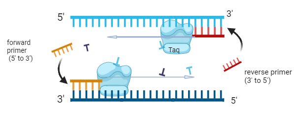
Picture made with BioRender

The temperature rises again to 72°C in the elongation phase, to activate heat-resistant Taq DNA polymerase which synthesises new strands of DNA complementary to the target sequence by attaching dNTPs (deoxynucleotide triphosphates) from the ends of the primer. The PCR machine cycles this process by continuously changing the temperature for sufficient amplification.

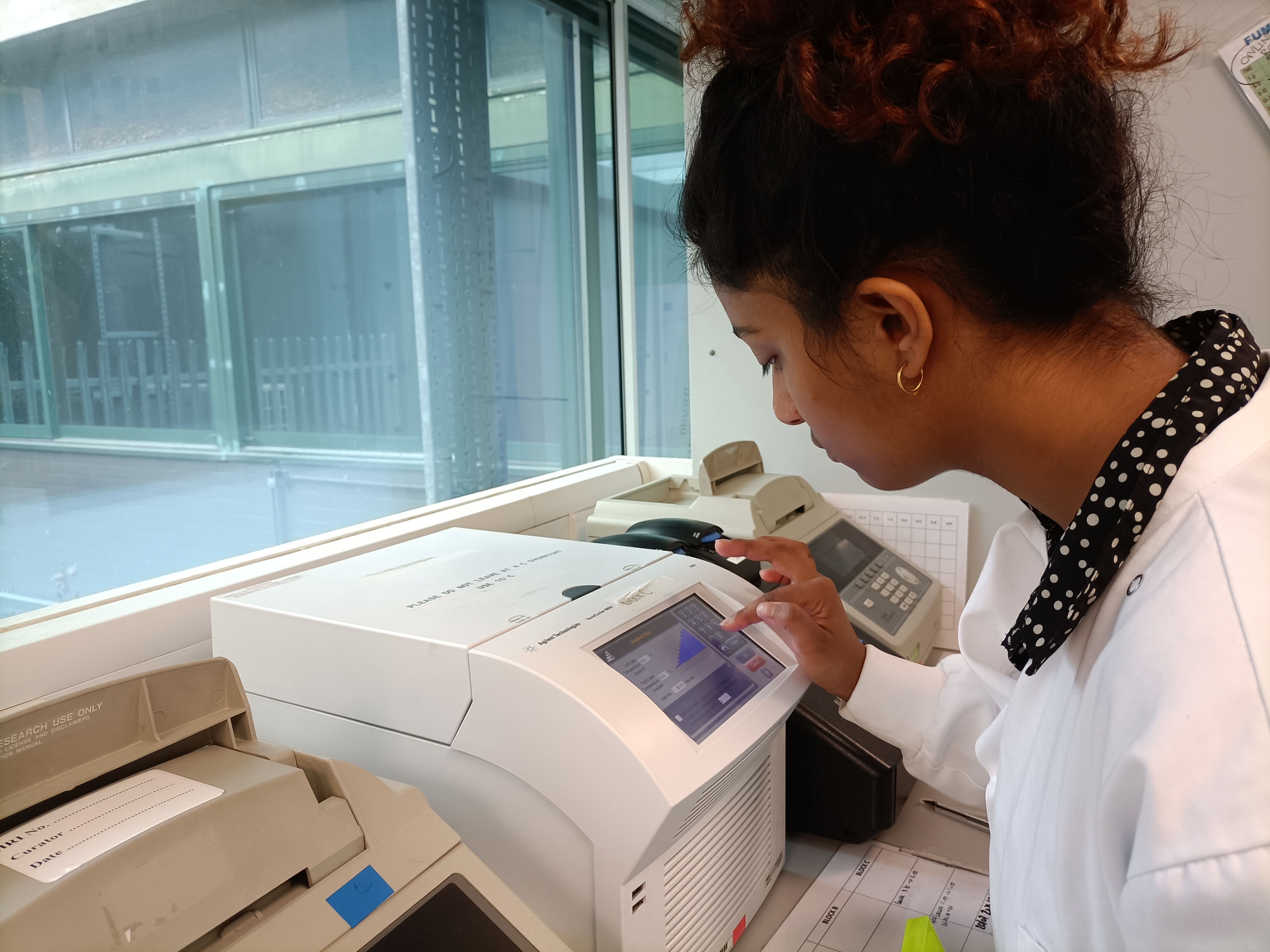
Here you can see me, setting the gradient step in the PCR machine.

During these two weeks, I used PCR to estimate the optimum annealing temperature for two unique sets of forward and reverse primers of mutant lines so we can genotype successfully later. I used a master mix known as BioMix Red which contains the Taq enzyme, dNTPs and MgSO₄ and buffer - in this way, I had to add only primers, wild-type DNA extractions made in the first two weeks and water. This mix is really useful to be able to check the presence of DNA analyses, but my goal is to be able to make a master mix with High-Quality Taq that can be used for cloning.

We have 7 lines left to genotype, every line has a couple of specific primers and I will run a separate gradient PCR for every primer set.

This is how it works: after placing my samples in the PCR machine, I need to add gradient step in the PCR program, which applies a range of annealing temperatures across the samples. The total reaction counts 35 cycles and lasts 1 hours and 30 mins. Afterwards, we run an agarose gel with our samples loaded onto it and an hour later we run a program called Gene Synthesis on a laptop that allows us to view DNA under UV light. The brighter the bands are on the image the better the primers have annealed hence that temperature should be selected for genotyping!

Back to the weekly journal

WEEK 5-6

Previously, I have been doing gradient PCR for different lines which told me what the optimum temperature is for the different primers. This is the temperature we set for the machine during the annealing phase of PCR. These weeks are about genotyping.

The purpose of genotyping is to confirm the presence of T-DNA in the required position and to confirm the status of my lines, in my case all the lines ordered should be homozygous.
T-DNA or transfer DNA insertion mutations can be used to identify the molecular mechanisms behind a particular biological process in plants. This is useful for us as by identifying mutant lines which have T-DNA in certain genes and using phenotypic comparison to the wild-type genotype, we can investigate which proteins are involved in the PTI and ETI response. Our mutant plants are known as SALK lines which are T-DNA insertion lines for the model plant Arabidopsis. Therefore to amplify this insertion using PCR we use the universal primer LBb1.3.
So, the protocol for this process is to create two master mixes, one is to identify the wild type only (Col0) and the other is for the mutant. The difference between the two master mixes is the primers, the master mix for the wild type will contain a forward and a reverse primer for the gene, whereas the master mix to identify the insertion will contain LBb1.3 and a reverse primer for the gene.
We will then produce two sets of samples, each set having the respective master mix. Both sets will have DNA extractions going from LCx (abbreviation for line) plant 1 to plant 6, the number of mutant plants included is a good sample size to be confident with the seeds received, Col0 as a positive control for the wild-type master mix and a negative control which replaces the same volume of DNA with water to check possible contamination.

The forward and reverse primers for the mutant line will only work in PCR if the T-DNA is not present since it’s too long (30Kb). These primers will be present in the wild-type master mix and therefore bands indicating that DNA is present once the gel has been run should only appear for Col0 DNA; the gene of interest does not have T-DNA. In the mutant master mix, we use the reverse primer for the line and a different primer which should anneal to the T-DNA so the bands of DNA that appear should be the entire mutant line and not Col0. No bands of DNA should appear for either negative control.

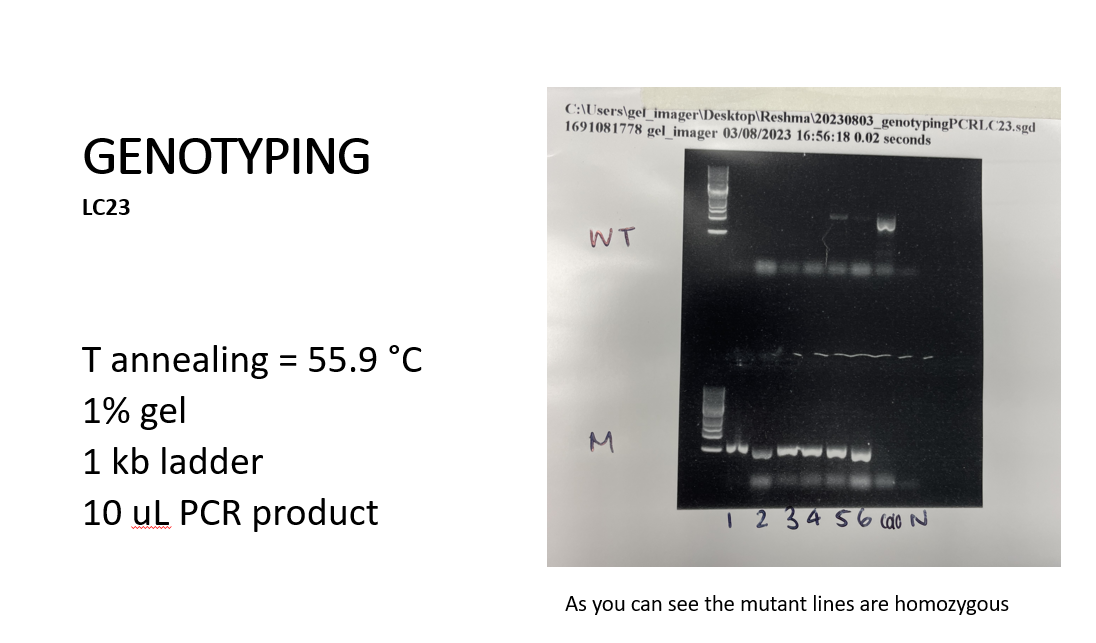
On the far left of the gel, we can see something that looks akin to a ladder this is called the 1 kb ladder which is used for all gels and is used to measure the total length of the DNA.

Back to the weekly journal

WEEK 7-8

After confirming the genotype of a mutant, we can move to phenotyping. Phenotyping infiltrated mutant plants allows us to observe the progression of disease in real-time. Usually, I start a phenotypic on a Tuesday to make the most out of phenotyping and I take pictures of my plants every morning and afternoon for the rest of the week. If one line is dying faster than the other, then this raises the possibility that the absence or knocked down of the gene is influencing plant immunity. To make this comparison between the different lines we needed to ensure that the plants were not dying too quickly; this was done infiltrating plants with bacteria at low concentrations, this is done using the OD measurement.

The bacteria that we chose to infect our plants with were DC3000 and HrpA. HrpA lacks the protein to deliver effectors to cause disease so can be used as a control to show that damage to the plants over time is caused by DC3000 and not by the infiltration technique. As mentioned in week 1-2 of my blog it is very easy to damage your plants when wounding and infiltrating them with bacteria. Therefore, if damage is seen in the leaves infiltrated with HrpA we can no longer conclude that the damage to the leaves infiltrated by DC3000 is because of symptoms of disease.

The night before infiltration we prepare our bacteria and leave them growing in an incubator (28*C is the best temperature for Pseudomonas!). To make an overnight we need plates of our bacteria; antibiotics which are stored in the lab’s fridge and vials of KB (liquid growth media) from the cold room. The antibiotics allow me to select the bacteria I want to grow, and any other bacteria will hopefully die since they lack the resistance for the antibiotics. DC3000 and HrpA require the antibiotics Rif and Kan. I then label my vial with the name of the bacteria and my name. Then I turn on Bunsen burner by turning the gas on and lighting it so that I can see a blue flame. This is done to keep my workplace sterile, so the unwanted bacteria do not grow.

I measure out 50 uL of Rif and 5 uL of Kan using the micropipettes into the vial and use a tip to swab the discrete, young colonies from the plates and drop the tips into the vials. THIS NEEDS TO BE DONE CLOSE TO THE FLAME! An extra thing you can do is hold up the tip to the flame (not in it) to ensure it is sterile. I will turn the Bunsen burner off once I am ready to put my vial in the incubator which should be shaking to ensure oxygenation of bacteria, so only when the lid of the vial is tightly screwed on.

The next morning it is time to run down our bacteria and see how much it has grown!

Whilst my bacteria are in a centrifuge for 7 minutes at 2800rpm I prepare a stock solution of 10mM MgCl₂ from 1M MgCl₂ (top tip for all my fellow undergraduate students C1V1 = C2V2 makes dilution calculations way less stressful). Once the bacteria have been run down, I tip out the solution and tip it into the waste contaminated liquids container. Then I transfer 10mL of 10 mM MgCl2 into the vial and shake it so the bacteria mixes with the solution. We then centrifuge again for the same amount of time and rpm and tip out the solution again except we are transferring 5mL of 10 mM MgCl2 now.

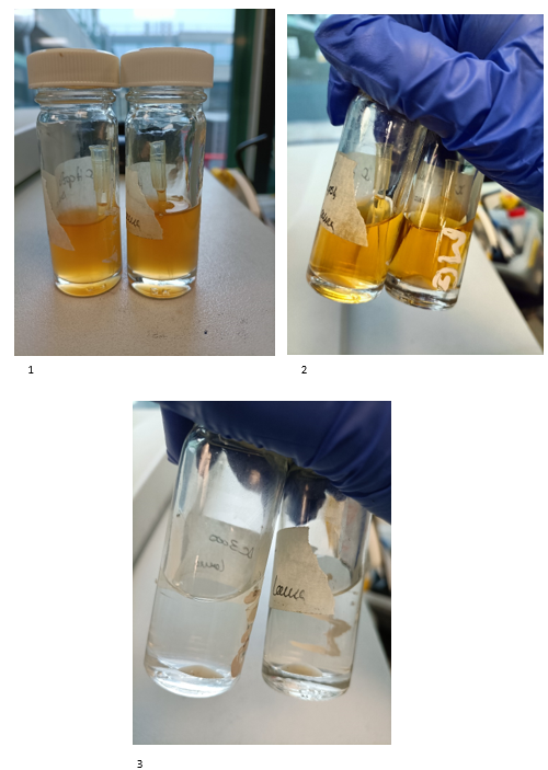
Here you can see different stages.

(1)  Bacteria have just been taken out of the incubator after one night at 28 degrees Celsius. 

(2)  The bacteria have been taken out of the centrifuge after 7 minutes, 2800 rpm and at room temperature. You can notice at the bottom of the flask bacteria.

(3)  At this point we have poured out the solution of antibiotics and replaced the vials with 10 ml of MgCl2. I have shaken it, so the bacteria have been suspended in solution and then I put it in the centrifuge for the same amount of time, rpm and temperature. And here they have been taken out of the centrifuge again. 

You can notice how the colour of the supernatant changes, this is really important since we are removing growth media and antibiotics that we don't want to infiltrate inside the plant.

We need to measure the concentration of the bacteria we have grown so we can use our best friend C1V1 = C2V2 equation to calculate the volume of distilled water required to dilute the bacteria to a desired concentration, in this case corresponding to OD = 0.05. A spectrophotometer quantifies the turbidity of the bacteria solution, so we use this machine to calculate the concentration. We need three cuvettes, one being a blank to calibrate the machine and the other for DC3000 and HrpA. Each cuvette should hold 1 ml of solution or 1000 microlitres. The blank would contain 1000 microlitres of MgCl2 and the other two would have 900 microlitres of salt and 100 microlitres of bacteria.

Using the spectrophotometer, we record the concentration of bacteria but multiply each respective value by 10 because we diluted by a tenth in the cuvettes. I micropipette the volume of bacteria I need from each vial into 15 ml tubes and then fill them up to 10 ml with my stock solution.

Now it’s time to infiltrate my plants!

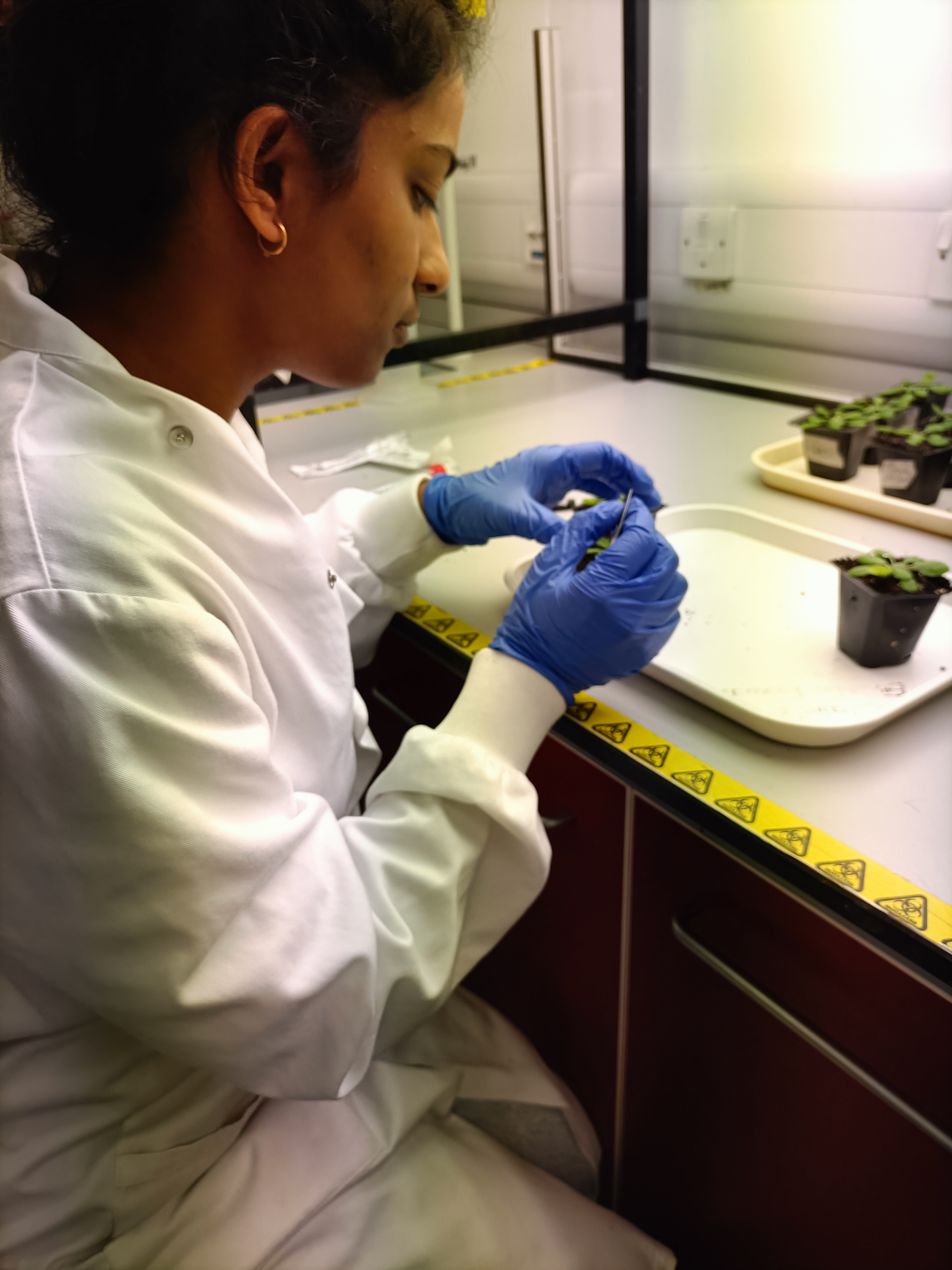
This is me wounding a plant using a razor blade.

Back to the weekly journal

WEEK 9-10

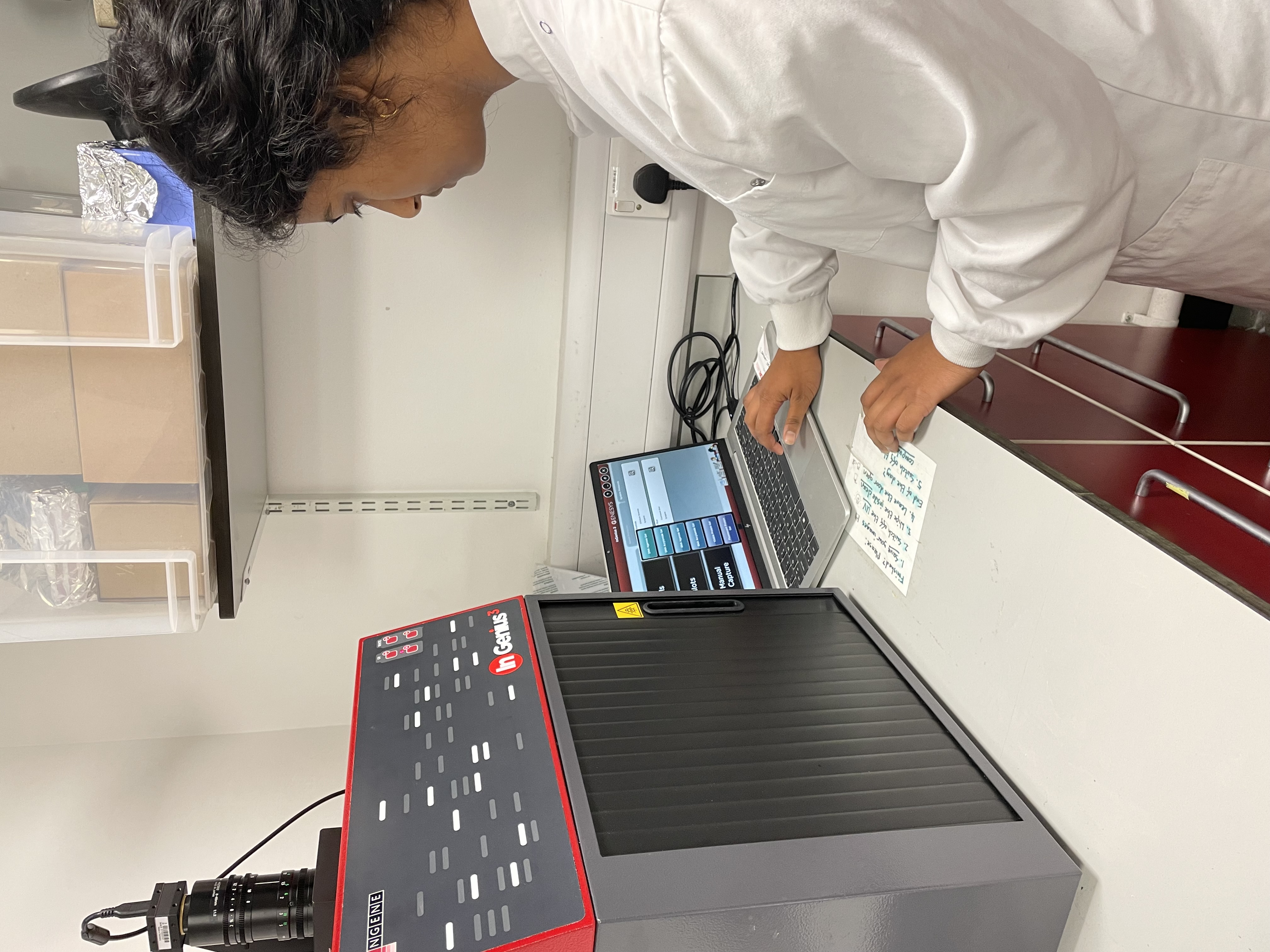
For the final part of my project, I imaged my infiltrated plants using fluor imaging cameras for a more detailed analysis of the interaction of effectors and proteins during the innate immune response in a plant. I needed to repeat making overnights and running down bacteria, but I prepared the bacteria solution at a concentration of 0.15 instead for camera analysis. We can run different software to analyse the images depending on the camera. Fluor images will quantify the progression of disease in the form of pixels. The data we are interested in is Fv/Fm which is a ratio of the variable fluorescence by maximum fluorescence produced by PSII, essentially, we are measuring the efficiency of PSII. Chlorophyll fluorescence is a light that is re-emitted at a longer wavelength after chlorophyll pigments absorb the light at a shorter wavelength, the shorter the wavelength the more energy it contains. An Fv/Fm value in the range of 0.79 to 0.84 is the approximate optimal value for many plant species with lowered values suggesting stress so this metric tests whether plant stress affects PSII in a dark, adapted state. Pathogenesis would trigger specific reactions in the plant causing a decline in photosynthesis which is a form of plant stress.

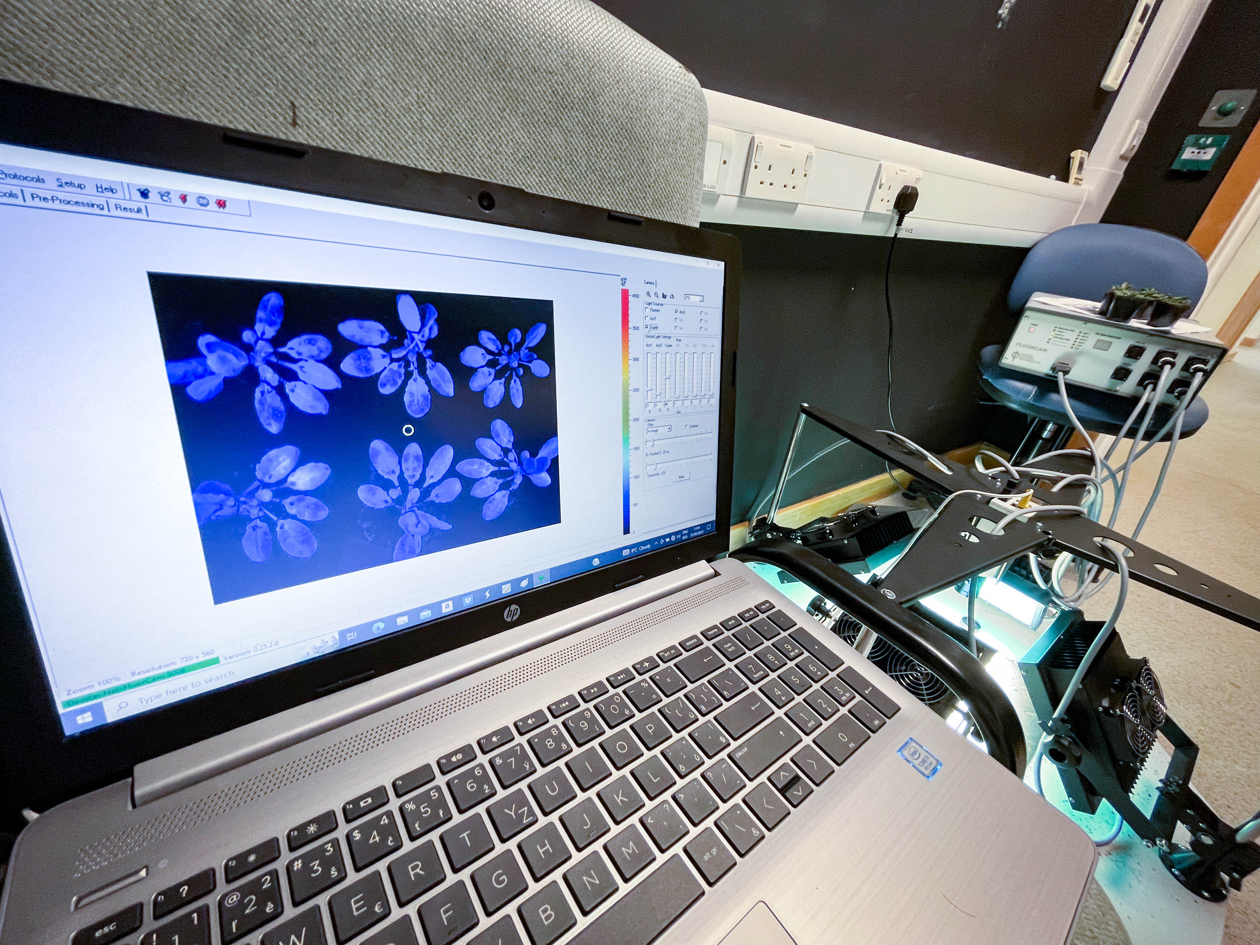
Here is the camera I used to image the infiltrated plants.

Variable chlorophyll fluorescence is only observed in chlorophyll a (specific type of pigment) in PSII I let the camera run for 24 hrs and every hour we capture the FV/FM value.

To analyse our results, we transfer the data onto Excel for each individual leaf we have infiltrated, we have six repeats for the same line and DC 3000 and two repeats for the same line and HrpA. We then find averages for FV/FM for each hour over 24 hours. This can be done using a formula in Excel.

To get a holistic overview of the results I created a line graph and compared the trend lines in the decline for FV/FM from 0.8 to 0.4, the rate of decline depends on a combination of the line and bacteria.

The fluor imaging cameras upstairs and in the lab have different requirements to be able to image infiltrated plants effectively. For example, we need to adjust the focus and aperture on the camera downstairs to get clear images and we need to turn off act2 manually, so the plants are in a dark-adapted state. When act2 is on the plants are flooded with bright light so you can see the plants on the camera whilst positioning them.

For the data presentation PowerPoint, I will read some literature to suggest a biological explanation for the different trends in the Fv/Fm for the different mutants.

Back to the weekly journal

PLANT MANAGEMENT

In this section, I would like to cover all the different activities we carried out in PBF, such as sowing, pricking, harvesting seeds etc.

First of all, I needed to sow my Arabidopsis lines. This is done by getting a pot full of specific soil without pressing it and rinse it with water, after that, I just need to tip some seeds from the Eppendorf onto the soil. This part is critical, I need to label every pot with the line sowed in and the date of sowing - never forget to sow the wild-type line for comparison!

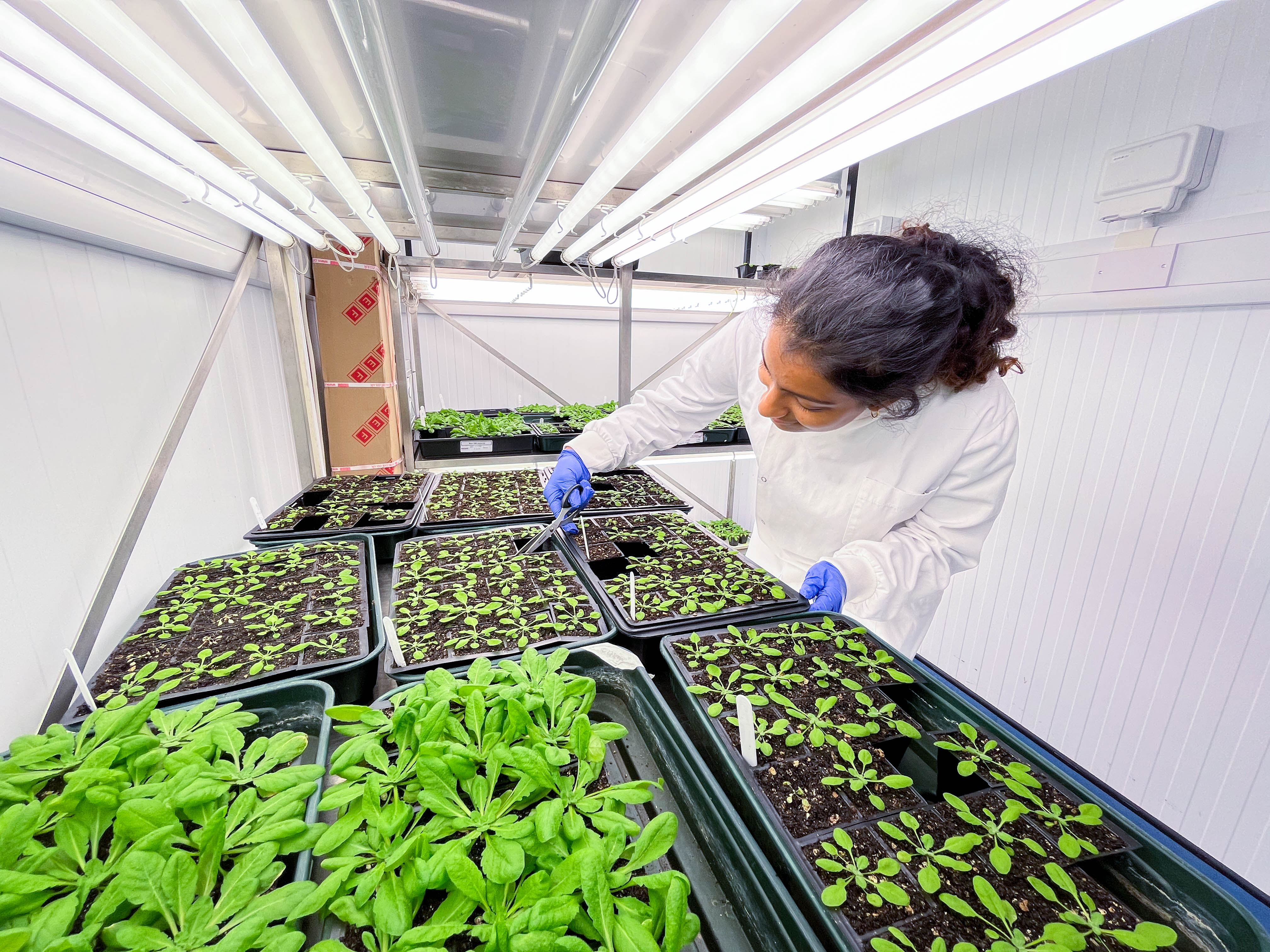
After 2 weeks, the plants are ready to be pricked. The pricking of these plants is essentially the second stage of growing your line of Arabidopsis. To start we filled a tray of pots with soil and pressed it down with our fingers to make room for more soil until it was no longer possible to do so. The soil we were using had chemicals such as pastiches, so gloves had to be worn; also, it’s never fun to get dirt under your fingernails. The next step was the irrigation of the soil which required cutting a pot out so we could pour a litre of water from a separate glass container into the tray. We then waited for all the soil to turn darker shade which indicated that it has absorbed the water. Then we placed a label in the soil that had the line of the plant, the date it was sowed and pricked written on it. At this point, we were ready to start pricking!
Using tweezers, we made a hole (the size of a finger tip) in each plant pot to place the seedling; the ideal seedling had to have 2 large and 2 small leaves and most importantly we needed to keep the root intact so that it could grow! Once pricking was over we placed a lid on the tray to maintain humidity and placed it in the storage facility of PBF.

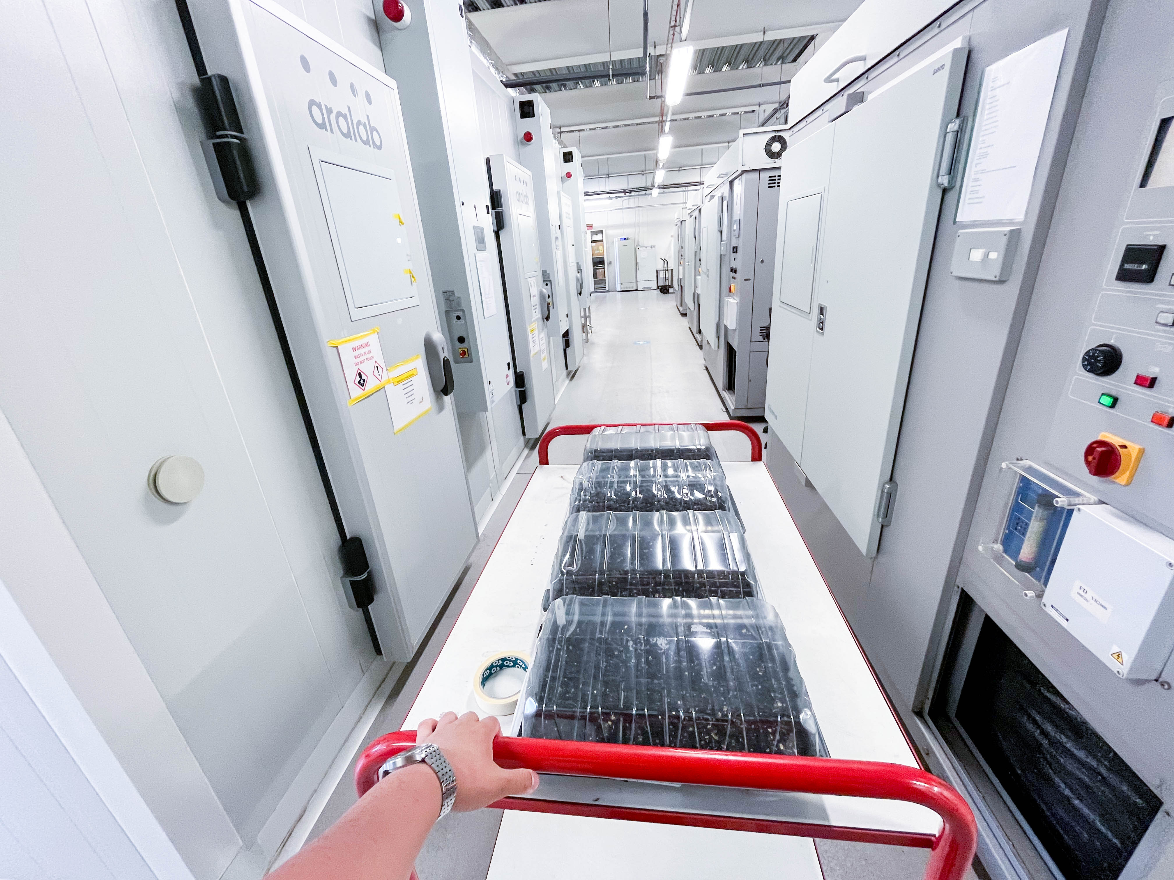
In this photo you can see some Arabidopdisis plants just pricked and move to the growth room.

Another activity I have performed in PBF is the harvest of Arabidopsis seeds. If there is a particular line of interest that we want to investigate further, a few seeds are never enough! To collect more seeds, I first bagged the plant I wanted to grow and let it flower, self-pollinated and dry up. When the siliques are dry, it's really important to separate the different lines of seeds, so I labelled small vials with the plant line and plant number (LC25 P1). Next, I cut the part of the plant that has flowered by the stem and threw away the remaining plant and packaging in an autoclave bag.
Working in a cabinet that controls airflow, I placed the dry upper part of the plant on a sieve, the sieve is placed on a horizontally positioned A4 sheet of paper that has previously folded in half. I then broke up the plant into smaller pieces to help filter the sieve and then transferred the seeds through the sieve again to make sure that everything is filtered properly and I don't have any plant residues - this can be done with the help of an additional sheet of paper. I repeated this process until I could no longer filter out the remaining parts of the plant from the seeds.
Putting the sieve to one side, I transferred the seeds using one A4 paper to the previously labelled vial which is on the second piece of paper; this process will be repeated until no more seeds end up in the vial.
The remaining seeds that cannot be transferred need to be removed so that the seeds are not mixed up with each other in the vials when this technique is repeated using a different line.

Back to the weekly journal