
Machine Learning in Astronomy
Intro
This page has a few examples of where I have implemented Machine Learning for Astro application:
Classifying White Dwarf Spectra
White Dwarfs show off their atmospheric composition through absorption. A process in which particular wavelengths of light are absorbed due to the presence of particular elements. We classify White Dwarfs on the elemental abundance in their atmospheres; which is based on the strength of absorption lines at certain wavelengths.
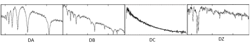
WD Spectal types
Atmospheres can show abundances of more than two elements. For example, a Hydrogen dominated atmosphere with traces of Helium would be catagorised as a DAB type.
Instead of training a computer to read the spectra and classify from that, it is faster and more accurate to paramatise the data. A way to do this is by modelling a featureless spectrum (i.e. what the White Dwarf would look like if it were DC type) and overlaying it on the original. By integrating at key absorption points, the area of the absorption lines are obtained (which can be considered strength of absorption). This is a supervised training method, the classifications are fed in to the machine learner with their corresponding areas calculated prior. It was found that the best classifier type for this problem is a random forest. Singular element types (DA, DB, DZ) have very good agreement with roughly 89-94% accuracy. CVs have a higher success rate ~98%, this is probably due to the emission lines making them distinct. The method struggles deeply with finding multi-class objects (DABs, DAZs, etc.) with a hit rate of only 40%, this may be because there are a large number of single element white dwarfs in the training sample resulting in a bias when training them.
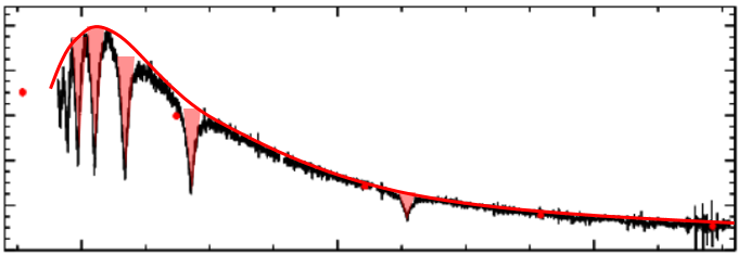
The red curve is a featureless fit, the red triangles represent the area found from integrating at absorption points.
Methods like these need to be developed, in the near future a swath of spectroscopic surveys (WEAVE, DESI, 4MOST) will be conducted collecting millions of White Dwarf spectra. Most of these targets will already be classified, however with more detailed data, their type may need to be updated and astronomers certainly won't have time to look at all of them.

Real or Bogus?
Some astronomers are only intretsed in looking at explosions in the night sky. These events evolve quickly and are relatively short lived. The challenge is to spot them quickly so we can do more detailed observations. The main way we do this is through image subtraction. A problem occurs that some of the residuals found through this method are false positives (Bogus!). We can implement a simple machine learner to tell the difference between a real detection and a bogus one!
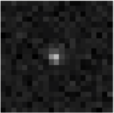
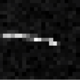
Real source, Fake source
This is an unsupervised learning method. We give the features of the detection to our classifier and it will create it's own catagories based on the features we give it. First, the features need to be defined. One of the most telling characteristics is the Zernike Distance. Zernkie Distance is based off the coefficients
 found when modelling the Zernike Polynomials of the stars found in the reference image from the subtraction process. On the right is a picture of a kitten which is being modelled using Zernike Polynomials. Each frame is a plot of the next orders coefficients. We can do the same with stars from telescope images. Because sources should have similar point spread functions, their Zernike Distance should be close to 0. This also means bogus sources will have distances much greater than 0. Another feature that can be added is the Scorr value from the ZOGY subtraction. This is a statistical score of how likely the residual is to be a change in the field.
There are two front runners for classifier methods. Bayes and Random Forest. The former offers more true positives, however it also lets a lot more false positives in. The exact opposite is true for Random Forest, fewer true positives with very few false positives. Depending on the scientist depends on which is more convenient. Deep learning may offer even more accurate real bogus
LSST Data challenge
Recently, Kaggle launched the PLAsTiCC Astronomical Classification challenge. In this challenge, synthetic photometric data needs to be classified.
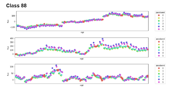
Example of the Challenge data
The data came in two main distinctions: Intergalactic (Z=0) and Extra-galactic(Z>0). By splitting the data, two neural nets were made for each scenario. We found applying a multi band Lomb-Scargle to the Z=0 data offered a strong training sample. In fact the confidence of the intergalactic sample shows to have a confidence of ~98%
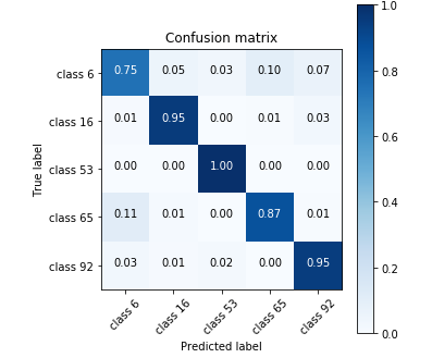
Confusion matrix of intergalactic data
The primary weakness was determining useful features from the extra-galactic data. Using the meta-data and a few curve features with Gaussian process regression, a basic neural net found an accuracy of roughly 70%.
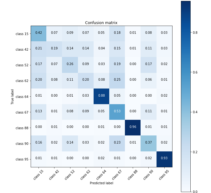
Confusion Matrix for Extra-galactic data
This weakness was the downfall of our submission, but hopefully this kind of photometric classification can be applied to GOTO data in the future.